findfeatures
Feature-based matching algorithms used to create ISIS control networks
Introduction
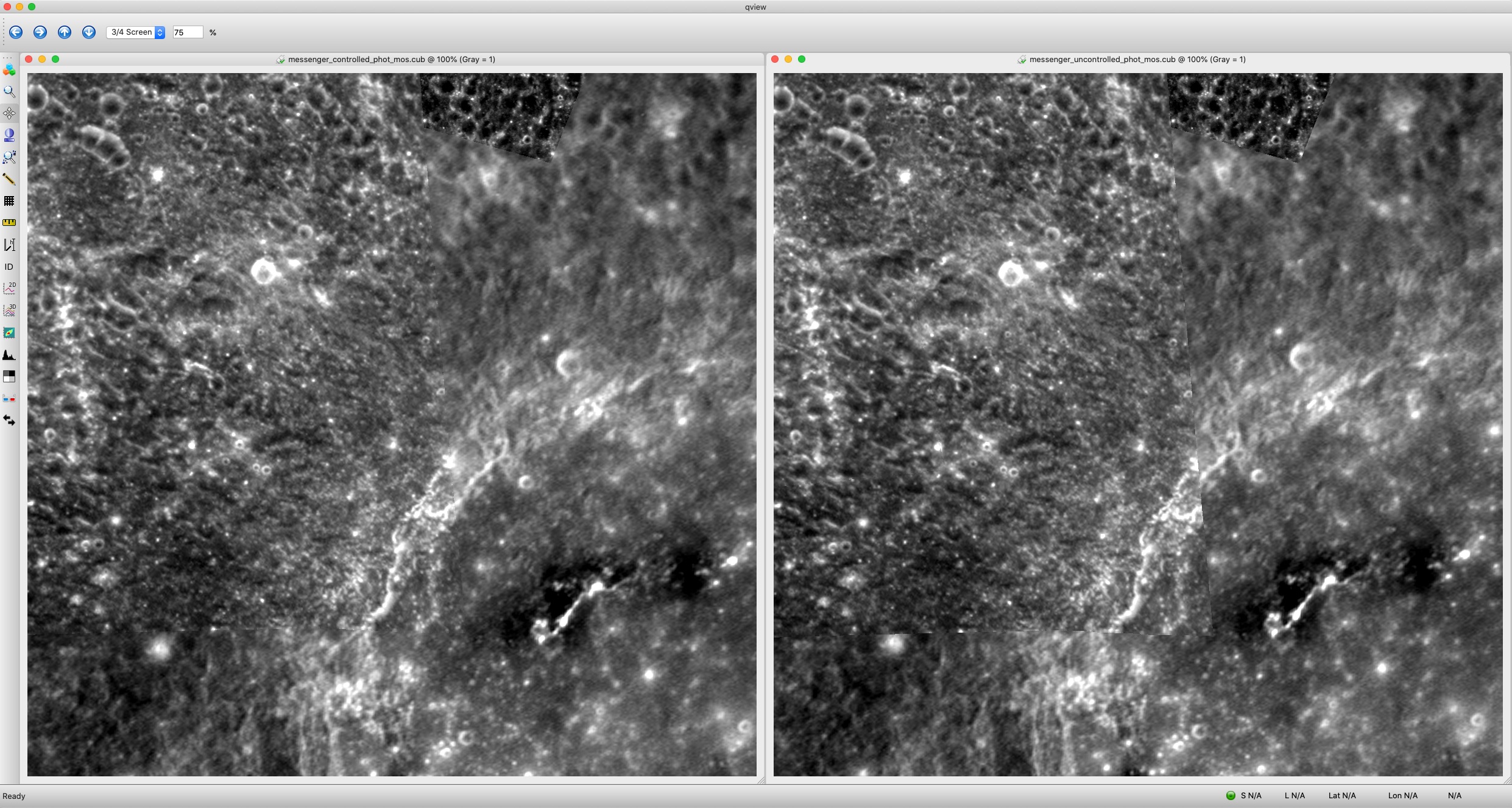
findfeatures was developed to provide an alternative approach to create image-based ISIS control point networks. Traditional ISIS control networks are typically created using equally spaced grids and area-based image matching (ABM) techniques. Control points are at the center of these grids and they are not necessarily associated with any particular feature or interest point. findfeatures applies feature-based matching (FBM) algorithms using the full suite of OpenCV detection and descriptor extraction algorithms and descriptor matchers. The points detected by these algorithms are associated with surface features identified by the type of detector algorithm designed to represent certain characteristics. Feature based matching has a twenty year history in computer vision and continues to benefit from improvements and advancements to make development of applications like this possible.
This application offers alternatives to traditional image matching options such as autoseed, seedgrid and coreg. Applications like coreg and pointreg are area-based matching, whereas findfeatures utilizes feature-based matching techniques. The OpenCV feature matching framework is used extensively in this application to implement the concepts commonly found in robust feature matching algorithms and applied to overlapping single pairs or multiple overlapping image sets.
Overview
findfeatures uses OpenCV's FBM algorithms to match a single image, or set of images, called the trainer image(s) (FROM/FROMLIST) to a different image, called the query image (MATCH).
Feature based algorithms are comprised of three basic processes: detection of features (or keypoints), extraction of feature descriptors and finally matching of feature descriptors from two image sources. To improve the quality of matches, findfeatures applies a fourth process - robust outlier detection.
Feature detection is the search for features of interest (or key points) in an image. The ultimate goal is to find features that can also be found in another image of the same object or location. Feature detection algorithms are often refered to as detectors.
Detectors describe key points based on their location in a specific image. Feature descriptors allow features found by a detector to be described outside of the context of that image. For example, features could be described by their roundness or how much they contrast the surrounding area. Feature descriptors provide a way to compare key points from different images. Algorithms that extract feature descriptors from keypoints in an image are called extractors.
The third process is to match key points from different images based on their feature descriptors. The trainer images can be matched to the query image (called a trainer to query match) or the query image can be matched to the trainer images (called a query to trainer match). findfeatures performs both a trainer to query match and a query to trainer match. Algorithms for matching feature descriptors are called matchers.
The final step is to remove outlier matches. This helps improve the quality and accuracy of matches when conditions make matching challenging. findfeatures uses a four step outlier removal process. At each step, matches are rejected and only the surviving matches are used in the following step.
- A ratio test comparing the best and second best match for each point removes points that are not sufficiently distinct.
- The matches are checked for symmetry. If a match was made in the trainer to query match, but not in the query to trainer match (or vice versa) then the match is removed.
- The fundamental matrices between the trainer images and the query image are computed using the RANSAC algorithm and matches that exceed the RANSAC tolerance are removed.
- The homography matrices (projections from one image's perspective into another) from the query image to the trainer images are computed using the RANSAC algorithm and matches with a high residual are removed.
Matches that survive the outlier rejection process are converted into an output control network. From here, multiple control networks created by systematic use of findfeatures can be combined into one regional or global control network with cnetcombinept. This can result in extremely large control networks. cnetthinner can be used to reduce the size of the network while maintaining sufficient distribution for use with the jigsaw application. If the control network is going to be used to create a DEM, then it should not be thinned.
Supported Image Formats
findfeatures is designed to support many different image formats. However, ISIS cubes with camera models provide the greatest flexibility when using this feature matcher. ISIS cubes with geometry can be effectively and efficiently matched by applying fast geometric transforms that project all overlapping candidate images (referred to as train images in OpenCV terminolgy) to the camera space of the match (or truth) image (referred to as the query image in OpenCV terminology). This single feature allows users to apply virtually all OpenCV detector and extractor, including algorithms that are not scale and rotation invariant. Other popular image formats are supported using OpenCV imread() image reader API. Images supported here can be provided as the image input files. However, these images will not have geometric functionality so support for the fast geometric option is not available to these images. As a consequence, FBM algorithms that are not scale and rotation invarant are not recommended for these images unless they are relatively spatially consistent. Nor can the point geometries be provided - only line/sample correlations will be computed in these cases.
Note that all images are converted to 8-bit when read in.
Specifications for Robust Feature Matching Algorithms
Robust matcher algorithms consist of detectors, extractors, and
matchers components and their parameters and are selected by a
specification string provided in the ALGORITHM parameter.
More that one matcher algorithm configuration can be provided in
a file, one algorithm per line, specified in the ALGOSPECFILE
parameter. The basic scheme is shown below (optional portions are
enclosed by [ ]).
detector[@param1:value1@...]/extractor[@param1:value@...][/matcher@param1:value1@...][/parameters@param1:value1@...]
The specification string consists of between two and four algorithm
matching components, such as detectors, extractors and matchers,
separated by /. Each algorithm component can also have
unique parameter entries separated by @. The first
algorithm component of the specification
string, detector[@param1:value1@...], defines the
detector. The first entry is the name of the algorithm. The remaining
entries are detector parameters separated by @ and define
values for the detector. The parameter specification consist of the
parameter name followed by : providing the parameter value.
After the detector algorithm and its parameters is / which
begins the extractor algorithm specification,
extractor[@param1:value@...]. Following the extractor
specification is another / and the matcher algorithm,
[matcher@param1:value1@...]. The extractor and matcher
specifications are formatted the same way as the detector component. The
final component of the specification string,
[/parameters@param1:value1@...] defines the robust matcher
parameters. The first entry is the word parameters. The
remaining entries consist of parameter name:value pairs,
just like the parameters in the algorithm specifications.
An alternative scheme for the specification string allows the
components to be in any order. Each component is formatted the same,
except the first entry in the detector, extractor, and (if specified)
matcher components begin with detector.,
extractor., and matcher. respectively. For
example, the specification below would enable root sift in the outlier
detection, define a FAST detector, a LATCH descriptor extractor,
and a FlannBased matcher.
extractor.LATCH@Bytes:16@HalfSSDSize:4/parameters@RootSift:true/matcher.FlannBasedMatcher/detector.FAST@Threshold:9@NonmaxSuppression:false
Many FBM algorithms are designed to use a specific detector, extractor
pair with shared parameters (SIFT and ORB are good examples of this).
For these cases, the alternative specification scheme allows for the
detector and extractor to be defined in a single component with shared
parameters. To do this, begin the first entry with
feature2d.. For example, the following specification would
define a SIFT algorithm with 4 octave layers for both the detector and
extractor along with a brute force matcher using the L1 norm.
matcher.BFMatcher@NormType:Norm_L1/feature2d.SIFT@NOctaveLayers:4.
The minimum specification string consists of a detector name and an
extractor name. When no matcher is specified, a brute force matcher
with parameters tailored to the extractor is used. For example
SIFT/SIFT would result in SIFT being used for the
detector, SIFT being used for the extractor, and a brute force matcher
used for the matcher. If used with the alternative specification
scheme, the detector and extractor can be defined in a single
component. So, the specification feature2d.SIFT defines
the exact same detector, extractor, and matcher as the previous
specification.
Multiple sets of FBM algorithms and robust matcher parameters can be entered via the ALGOSPECFILE parameter. It takes a text file (*.lis) with a specification on each line. For each specification, a separate set of FBM algorithms and robust matcher parameters will be created. Each set will be used to match the input images and the set that produces the best matches will be used to create the output control network. When the DEBUG and/or DEBUGLOG parameters are used, the results from each set along with the quality of the match will be output.
Each algorithm has default parameters that are suited for most uses. The LISTALL parameter will list every supported detector, extractor, and matcher algorithm along with its parameters and default values. The LISTSPEC parameter will output the results of the parsed specification string(s). A description of every algorithm supported by findfeatures and if they can be used as a detector, extractor, and/or matcher can be found in the Algorithms table.
Descriptions of the robust matcher parameters and their default values can be found in the Robust Matcher Parameters table.
Choosing Feature Matching Algorithms
Choosing effective algorithms and parameters is critical to successful use of findfeatures. If a poor choice of algorithms and/or parameters is made, findfeatures will usually complete, but excessive computation time and/or poor quality control network will result. findfeatures supports all of the OpenCV detectors, extractors, and matchers. Some algorithms work well in a wide range of scenarios (BRISK and SIFT are both well tested and very robust), while others are highly specialized. The following section provides guidelines to determine which algorithms and parameters to use.
findfeatures gives users a wide range of options to alter algorithms functionaility. Such a broad range of choices/combinations can be intimidating for users who are unfamiliar with FBM. The following are some suggestions to help make reasonable decision. First, when in doubt, trust the defaults. The defaults in findfeatures are designed to be a reasonable choice for a wide range of conditions. They may not be suitable for every situation but special configurations are usually not required to produce acceptable results. Defaults for the detector and extractor algorithms are not provided, but the SIFT algorithm is a very general, scale and rotation invariant, robust algorithm that can produce high quality control networks for most situations. The majority of more modern algorithms are focused on speed and efficiency.
If at all possible, always use the FASTGEOM parameter. The majority of problems when using FBM arise when trainer and query images have inconsistent spatial geometry and/or significant variations in observing conditions during image acquisition. The FASTGEOM parameter helps minimize these challenges by using a priori ephemeris SPICE data to create and apply a perspective matrix warp projection using the query and training geometry. Combining the FASTGEOM option with algorithms that are designed for speed (the FAST descriptor and BRIEF extractor are reasonable options) will quickly produce a control network. Keep in mind these networks are whole-pixel accuracy and will likely require refinement to subpixel accuracy with pointreg prior to bundle adjustment with jigsaw.
Different detectors search for different types of features. For example, the FAST algorithm searches for corners, while blob detection algorithms search for regions that contrast their surroundings. When choosing which detector to use, consider the prominent features in the image set. The FAST algorithm would work well for finding key points on a linear feature, while a blob detection algorithm would work well for finding key points in nadir images of a heavily cratered area.
When choosing an extractor there are two things to consider: the invariance of the extractor and the size of the extracted descriptor. Different extractors are invariant (i.e, not adversely affected) to different transformations. For example, the SIFT algorithm uses descriptors that are invariant to rotation, while BRIEF feature descriptors are best for images that are spatially similar in orientation. In general, invariance to more transformations comes at a cost, bigger descriptors. Detectors often find a very large number of key points in each image. The amount of time it takes to extract and then compare (i.e., match) the resultant feature descriptors heavily depends upon the size of the descriptor. So, more invariance usually means longer computation times. For example, using the BRIEF extractor (which extracts very small feature descriptors) instead of the SIFT extractor (which has moderately sized feature descriptors) provides an order of magnitude speed increases for both extraction and matching. If your images are from similar sensors and under similar conditions, then an extractor that uses smaller descriptors (BRISK, BRIEF, etc.) will be faster and just as accurate as extractors that use larger, more robust descriptors (SIFT, etc.). If your images are from very different sensors (a line scanner matched to a highly distorted framing camera, a low resolution framing camera and a high resolution push broom camera, etc...) or under very different conditions (very oblique and nadir, opposing sun angles, etc.) then using an extractor with a more robust descriptor will take longer but will be significantly more accurate than using an extractor with a smaller descriptor.
findfeatures has two options for matchers: brute force matching and a FLANN based matcher. The brute force matcher attempts to match a key point with every key point in another image and then pairs it with the closest match. This ensures a good match but can take a long time for large numbers of images and key points. The FLANN based matcher trains itself to find the approximate best match. It does not ensure the same accuracy as the brute force matcher, but is significantly faster for large numbers of images and key points. By default findfeatures uses a brute force matcher with parameters automatically chosen based upon the type of extractor used.
Several parameters allow for fine tuning of the outlier rejection process. The RATIO parameter determines how distinct matches must be. A ratio close to 0 will force findfeatures to consider only unambiguous matches and reject a large number of matches. If many, indistinct features are detected in each image, a low ratio will result in smaller, higher quality control networks. If few, non-distinct features are detected in each image, a high ratio will prevent the control network from being too sparse. The EPITOLERANCE and EPICONFIDENCE parameters control how outliers are found when the fundamental matrices are computed. These parameters will have the highest impact when the query and trainer images are stereo pairs. The HMGTOLERANCE parameter controls how outliers are found after the homography matrices are computed. This parameter will have the highest impact when the query and trainer images have very different exterior orientations. When using FASTGEOM, it is recommended to use higher values for these tolerances due to distortions that are introduced by image size perspective warping using the homography matrix.
Prior to FBM, findfeatures can apply several transformations to the images. These transformations can help improve match quality in specific scenarios. The FASTGEOM, GEOMTYPE, and FASTGEOMPOINTS parameters allow for reprojection of the trainer images into the query image's geometry prior to FBM. (This algorithm is very similar to processing by the ISIS cam2cam application. FASTGEOM differs in that it is not as robust or accurate as cam2cam because FASTGEOM applies a single matrix to warp the entire image - cam2cam uses a rubber sheet projection which is significantly more robust and accurate but can take significantly longer to project images.) These parameters can be used to achieve the speed increases of algorithms that are not rotation and/or scale invariant (BRIEF, FAST, etc.) without loss of accuracy. These parameters require that the trainer and query images be ISIS cubes with geometry/cartography capabilites established by running the spiceinit application on all images. For rotation and scale invariant algorithms (SIFT etc.), these parameters may have very little or significant adverse effects.
The FILTER parameter allows for the application of filters to the trainer and query images prior to FBM. The SOBEL option will emphasize edges in the images. The Sobel filter can introduce artifacts into some images, so the SCHARR option is also available to apply a more accurate filter. These filters allows for improved detection when using edge based detectors (FAST, AGAST, BRISK, etc...). If an edge based detector is not detecting a sufficient number of key points or the key points are not sufficienty distinct, these filters may increase the number of successful matches.
The OpenCV methods used in the outlier rejection process have several options that can be set along with the algorithms. The available parameters for are robust matcher algorithms are listed in the following Robust Matcher Parameters table. Feature matching algorithms and their descriptions and references are listed in the Algorithms table. The LISTALL program option will list all available algorithms, their feature capabilities, and parameters with default values.
| Keyword | Default | Description |
|---|---|---|
| SaveRenderedImages | False | Option to save the images that are matched after all transforms (e.g., fast geom, filtered, etc...) have been applied. The query (MATCH) image will have "_query" will be appended to the base name. All FROM/FROMLIST images will have "_train" appended to their names. They are saved as PNG images in the directory specifed by the SavePath parameter. |
| SavePath | $PWD | Specify the directory path to save all transform rendered images if SaveRenderedImages=TRUE. |
| RootSift | False | Apply the RootSift algorithm to the descriptors that normalizes SIFT-type of descriptors. A good description of the application of this algorithm is described in this article. In general, SIFT descriptors histograms are compared in Euclidean space. RootSift applies a Hellinger kernel to the descriptor histograms that greatly improve performance and still allows Euclidean distances in its evaluation. Be sure to use this for SIFT-type descriptors only. |
| MinimumFundamentalPoints | 8 | The Epipolar algorithm in OpenCV requires a minimim of 8 points in order to properly compute the fundamental matrix. This parameter allows the user to specify the minimum number of points allowed. |
| RefineFundamentalMatrix | True | A single computation of the fundamental matrix is performed unless this parameter is set to true. In this case, a new fundmental matrix is computed after outlier are detected and removed. This will improve the matrix since outliers are removed and the matrix is recomputed. |
| MinimumHomographyPoints | 8 | As in the Epipolar fundamental matrix, a minimum number of 8 points is required to compute the homography matrix for outlier detection. This parameter allows the user to specify a new minimum. |
| Name | Algorithm Type | Description | Further Reading |
|---|---|---|---|
| AGAST | Detector | The AGAST algorithm is a corner detection algorithm that builds on the FAST algorithm to detect features as quickly as possible. The main improvements are increased detection speed and less training time. | |
| Blob | Detector | A simple blob detection algorithm that attempts to identify connected components of the image based on DN values. The Blob algorithm is able to filter features after detection based on their characteristics. | |
| FAST | Detector | The FAST algorithm is a corner detection algorithm that is designed to detect corners extremely quickly. It uses machine learning to improve its accuracy. | |
| GFTT | Detector | The GFTT algorithm is based upon the Harris corner detector. The detection is based upon the idea that a corner varies significantly from all immediately adjacent regions. | |
| MSD | Detector | MSD stands for Maximal Self-Dissimilarities. It is based upon the idea that regions that vary significantly from their surroundings are easy to uniquely identify from different perspectives. The MSD algorithm detects generic features, so it is invariant to many image transformations and works well with stereo pairs. | |
| MSER | Detector | The MSER algorithm searches for regions which have significantly higher or lower intensity compared to their immediate surroundings. It works well for extracting features from images that lack strong edges. Because it depends upon intensity, MSER is very sensitive to factors such as solar angle and occlusion. In exchange MSER offers strong invariance to image geometry factors such, as resolution and emission angle (as long as features are not occluded). | |
| Star | Detector | The Star algorithm is OpenCV's implementation of the CenSurE algorithm which is fast and scale-invariant. It is a more robust version of the SIFT algorithm. | |
| AKAZE | Detector, Extractor | The AKAZE (accelerated KAZE) algorithm is a modified version of the KAZE algorithm which uses a faster method to compute non-linear scales. Like the KAZE algorithm, AKAZE works well for situations where the trainer and query images have different resolutions and possibly different distortions. AKAZE should be used over KAZE when strong invariance is needed but the size and/or number of images presents computation time concerns. The AKAZE algorithm can only be used as an extractor if either the KAZE or AKAZE algorithm was used as the detector. | |
| BRISK | Detector, Extractor | The BRISK algorithm uses concentric rings of points around features to extract a descriptor. It extracts a small, binary descriptor, so it is very fast. Unlike other binary descriptor extractors, BRISK offers moderate rotation invariance by use points far from the feature to determine orientation and then points close to the feature to determine intensity after accounting for the orientation. | |
| KAZE | Detector, Extractor | The KAZE algorithm is a very robust algorithm that attempts to provide improved invariance to scale. The method that SIFT use to provide scale invariance can result in proliferation of noise. The KAZE algorithm employs a non-linear scaling method that helps prevent this. Hence, the KAZE algorithm provides very strong invariance, but at the cost of large computation time. If very strong invariance is required but computation time is a concern, use the AKAZE algorithm instead. The KAZE algorithm can only be used as an extractor if either the KAZE or AKAZE algorithm was used as the detector. | |
| ORB | Detector, Extractor | The ORB algorithm extracts a very fast binary descriptor. It provides improved rotational invariance compared to BRIEF by accounting for orientation, but at the cost of slower extraction. It also attempts to learn the best way to extract information from around each feature. The ORB algorithm is faster than BRISK and FREAK, but provides less invariance. | |
| SIFT | Detector, Extractor | The SIFT algorithm is one of the oldest and most well tested FMB algorithms. It is a common benchmark for comparison of new algorithms. The SIFT algorithm offers good invariance, but can require large computation times. It is a good choice for both detector and extractor when a high quality output control network is needed and computation time is not a major concern. | |
| BRIEF | Extractor | The BRIEF algorithm extracts an extremely fast binary descriptor. If the query and trainer images are very similar, then the BRIEF algorithm offers unmatched speed. This speed comes at a cost, the BRIEF algorithm behaves very poorly if the query and trainer images vary significantly. The FASTGEOM parameter can help improve the quality of the match when using the BRIEF algorithm with varied query and trainer images. | |
| DAISY | Extractor | The DAISY algorithm is an adaptation of the extractor used by SIFT and SURF. It was designed for use with stereo imagery. The DAISY algorithm offers strong invariance similar to SIFT and SURF, but with significantly faster computation time. | |
| FREAK | Extractor | The FREAK algorithm extracts a fast binary descriptor. Like ORB, it attempts to learn the best way to extract information from around the features. The FREAK algorithm replicates how the human retina works attempting to produce tiered solutions. If the first solution does not provide uniqueness within a desired threshold, then a second, more precise solution is computed. The FREAK algorithm provides fast computation times along with adaptability to the requirements of the query and trainer images. | |
| LATCH | Extractor | The LATCH algorithm extracts a fast binary descriptor that offers greater invariance than other binary descriptor extractors. It lies between the extremely fast binary descriptor extractors (BRIEF and BRISK) and the very invariant but slow descriptor extractors (SIFT). The LATCH algorithm also offers a CUDA implementation that allows for extremely fast computation times when using multiple GPUs in parallel. | |
| LUCID | Extractor | The LUCID algorithm was designed to extract feature descriptors from color images. It offers invariance close to SURF and BRIEF with shorter computation times. | |
| BFMatcher | Matcher | The brute force matcher algorithm attempts to match the query and train images by brute force. It is guaranteed to find the best match, because it checks every match. For large numbers of features, this approach can require considerable computation time. | |
| FlannBasedMatcher | Matcher | The FLANN based matcher algorithm computes matches based on approximate nearest descriptors. It uses the FLANN library to learn how to approximate descriptor matches. The FLANN based matcher algorithm does not guarantee the best match for each feature, but will match large sets of features and/or images in significantly less time that the brute force matcher algorithm. When combined with outleir rejection, the FLANN based matcher algorithm can provide high quality matches. |
Customizing Feature Matching Algorithms
There are four options to select and customize Feature Matching algorithms and their parameters. The two findfeatures parameters that specify Feature Matching algorithms are the ALGORITHM and ALGOSPECFILE parameters. The ALGORITHM parameter accepts a string that adheres to the specifications as described above that select the detector, extractor and matcher algorithms. Parameters for each of those algorithms can be provided in the string as well. The ALGOSPECFILE parameter accepts the name of a file containing one or more Feature Matching algorithm configurations that also adhere to the specification.
The ALGORITHM and ALGOSPECFILE parameters should contain the full specification of the Feature Matching algorithms, including the optional "/parameters" of the algorithm. At times, its useful to alter this component of the algorithm to customize for each set of data without having to maintain seperate files (although maintaining specs in those file is recommended practice). The findfeatures ALGORITHM "/parameters" component of the feature matching specification command line overrides the contents of the file specified in the PARAMETERS program parameter. This allows runtime specification of mainly the ALGOSPECFILE PVL-type file contents to alter behavior of this component of the feature matching algorithm.
Initial values of outlier matching parameters that can be specified in the PARAMETERS program option can be found in the Robust Matcher Parameters table. Use of PARAMETERS excludes the need for these values to be specified in the command line without having to explicitly add them to the ALGORITHM string specification or ALGOSPECFILE.
The findfeatures GLOBALS program option allows users to specify "/parameters" keywords that are applied in the Feature Matching algorithms (as well as FASTGEOM algorithms). Individual parameters are specifed in accordance with the ALGORITHM string specification described above. For example, users can select to have all matched files saved as PNGs by specifying "GLOBALS=SaveRenderedImages:true". This allows the most convenient method to alter or fully specify feature matching parameters at runtime without having to edit or provide any parameterization files.
The order of precedence of Feature Matching parameterization is (lowest to highest) PARAMETERS, ALGOSPECFILE, ALGORITHM and finally GLOBALS.
The FASTGEOM Algorithm
The FASTGEOM option provides advanced geometric processing of training images (FROM, FROMLIST) before they are matched to the query (MATCH) image. The application of the FASTGEOM option is indicated when a wide variety of observation geometry is present in the FROM/FROMLIST images. Once applied, all OpenCV feature matching algorithms can be used particularly those that are not rotation and scale invariant. This is intended to provide a wide variety of feature matching options to users that result in better, and more comprehensive image control networks that contain more images with higher numbers of control points and higher density counts of control measures.
ISIS inherently provides all the necessary cartographic capabilities that make it possible to preprocess the images to eliminate, as much as possible, scale and rotation variances in images. By using a priori geometry provided by SPICE data, findfeatures constructs transformation matrices for each trainer image that matches the geometric properties of the query image. Applying the transformation matrix to each trainer image results in a (fast) projection, or warp, of the image into the image space of the query image, thus minimizing scale and rotation invariance. This defines the FASTGEOM processing objectives in findfeatures. Note that translation, or spatial offsets, may likely exist between images due to the inherent nature of a priori ephemeris data. This option is known to have problems with image sets of irregular bodies, especially for images acquired along the long axis of the target body..
The FASTGEOM algorithms requires all input images to have ISIS-based SPICE ephemeris applied by the spiceinit application. If any image does not have SPICE or no common latitude/longitude coordinates can be determined between the trainer image and the query image, they are exclude from feature matching and will be recorded in the TONOGEOM file. Feature matching will continue if one or more trainer image is successfully transformed.
Effective Use of FASTGEOM Algorithms
The FASTGEOM option provides two different algorithms - grid and radial - that can be used to associate common latitude/longitude coordinates between two images. These common latitude/longitude coordinates are translated to line/sample image coordinates in both images which are then used to create a homography 3x3 transformation matrix mapping the trainer line/sample coordinate pairs into the cooresponding query line/sample image coordinates. After the trainer images are read in, the homography transformation matrix is applied using a perspective warp projection of the trainer image. The GEOMTYPE parameter determines the type of output image is produced from the projection. This produces the projected trainer image that will be matched to the query image. The query image is not modified in this process.
Several common parameters govern behavior of both the grid and radial FASTGEOM algorithms. Note each algorithm is applied independently to every query/trainer image pair. For each image pair, the values used/computed and the resulting homography matrix are logged in the DEBUGLOG file (when DEBUG=true). The algorithm parameters are described in the following table.
| Keyword | Default | Description |
|---|---|---|
| FastGeomAlgorithm | Radial | Specifies the name of the FASTGEOM point mapping algorithm to use to compute common latitude/longitude and line/sample coordinates in the query and trainer images. Valid options are Radial and Grid. |
| FastGeomPoints | 25 | The minimum number of valid mapping points required in order to compute the homography image transformation matrix. If after the algorithm completes point mapping computations there are no FastGeomPoints valid points, the image is not added to the trainer match list and reported in TONOGEOM. The minimum value is 25, the maximum is all pixels in the images. |
| FastGeomTolerance | 3.0 | The maximum pixel outlier tolerance allowed in computing the homography matrix from query and trainer image mapped points generated from the FASTGEOM algorithms. The outlier for each mapping point is computed by using the homography matrix to translate each trainer point to the perspective query point and calculating the Euclidean distance from the actual query point. If the absolute distance is larger than FastGeomTolerance the point is rejected. Note the remaining inlier points are allowed to be less than FastGeomPoints. |
| FastGeomQuerySampleTolerance | 0.0 | This parameter allows the number of query image samples to exceed the actual number of pixels in the image FOV by this tolerance on both left and right boundaries of the image. This is intended to give the algorithms the best chance to collect the necessary number of mapping points to compute the homography tramsformation matrix. This value is not recommended to be too large, perhaps 5 - 10 pixels at the most. |
| FastGeomQueryLineTolerance | 0.0 | This parameter allows the number of query image lines to exceed the actual number of pixels in the image FOV by this tolerance on both top and bottom boundaries of the image. This is intended to give the algorithms the best chance to collect the necessary number of mapping points to compute the homography transformation matrix. This value is not recommended to be too large, perhaps 5 - 10 pixels at the most. |
| FastGeomTrainSampleTolerance | 0.0 | This parameter allows the number of trainer image samples to exceed the actual number of pixels in the image FOV by this tolerance on both left and right boundaries of the image. This is intended to give the algorithms the best chance to collect the necessary number of mapping points to compute the homography tramsformation matrix. This value is not recommended to be too large, perhaps 5 - 10 pixels at the most. |
| FastGeomTrainLineTolerance | 0.0 | This parameter allows the number of trainer image lines to exceed the actual number of pixels in the image FOV by this tolerance on both top and bottom boundaries of the image. This is intended to give the algorithms the best chance to collect the necessary number of mapping points to compute the homography tramsformation matrix. This value is not recommended to be too large, perhaps 5 - 10 pixels at the most. |
| FastGeomDumpMapping | false | This parameter informs the FASTGEOM algorithm to dump the mapping points of every query/trainer image pair to a CSV file. This will produce a file in the current directory of the form queryfile_trainerfile_{FastGeomAlgorithm}.fastgeom.csv where queryfile is the base name of the MATCH file with no directory or file extension, the trainerfile is the base name of the FROM/FROMLIST file with no directory or file extension, and {FastGeomAlgorithm} is the type of algorithm specified in that parameter. The columns written to the file are: QuerySample, QueryLine, TrainSample, TrainLine, Latitiude, Longitude, Radius, X, Y, Z, InTrainFOV. All values are floating point except InTrainFOV which is either True or False, True indicating the point is (valid) in both images. The name of this file is indicated in th DEBUGLOG file as PointDumpFile for eac query/trainer image pair. |
FASTGEOM Grid Algorithm
The FASTGEOM Grid algorithm computes a coreg-like rectangular set of grid points that are evenly space in each image axis. This algorithm will continue to refine the grid by decreasing the spacing between each iteration until at least FastGeomPoints valid mapping points are found. The algorithm continues to refine the spacing until every pixel in the query image is check for a valid mapping coordinate into the trainer image. Therein lies the potential for this algorithm to consume massive time and compute resources for images that contain very few or no valid common geometric points between query and trainer images. Therefore, some parameters are provided that place constraints/boundaries on the variables of this algorithm. These parameters are described in the following table.
| Keyword | Default | Description |
|---|---|---|
| FastGeomGridStartIteration | 0 | Specifies the starting iteration of the grid loop that calculates mapping points from query to trainer images. The first loop is 0 and it is computed so that it will be as close to the number of points specified in FastGeomPoints. It can start with any itertion less than or equal to FastGeomGridStopIteration. |
| FastGeomGridStopIteration | calculated |
Specifies the terminating iteration of the grid loop that calculates
mapping points from query to trainer images. The last loop, if not
specified by the user, is calculated as
max( max(query lines/samples), max(trainer lines/samples) ) / 2.0.
It is possible to specify no points if FastGeomGridStartIteration
is greater than FastGeomGridStopIteration.
|
| FastGeomGridIterationStep | 1 |
Specifies the iteration increment that is added to the current
iteration that is used to calculate the line/sample grid spaceing.
The actual grid spacing for line and sample axes are computed
as max( 1.0, queryAxisSize/(currinc*1.0)), where
queryAxisSize is the number of samples or lines in the axis and
currinc is increment + ( iteration * 2 ), where
iteration is the current increment + FastGeomGridIterationStep.
|
| FastGeomGridSaveAllPoints | false | At each new iteration in the grid algorithm, all points in the previous iteration are deleted. This true/false flag can be set to true to preserve all mapping points in earlier iterations. This may help in reaching the minimum FastGeomPoints but also runs the risk of duplicate points, thus biasing the homography matrix or creating an invalid matrix. This option is not recommended as it may create more problems than it resolves. |
This algorithm works best for high resolution images where there are little or no discontinuities in geometry and no limbs. It also can result in excessively long run times and/or significant computed resources for approach images where valid geometry is only in a small localized region in the image FOV. In those cases, the FASTGEOM radial algorithm is recommended.
FASTGEOM Radial Algorithm
The FASTGEOM Radial algorithm computes common geometric mapping points in the query and trainer images that are generated from a radial pattern originated at the center of the query image. The radial algorithm differs most from the grid algorithm because it is not iterative. It is a one shot algorithm where a single pattern is generated from parameters that are designed to provide a dense radial pattern. It can be much more efficient than the grid algorithm but runs a higher risk of failure due to underdetermination of sufficient number of common geometric points. This is the default algorithm if one is not specified by the user. The parameters that can be provided to customize the radial pattern created in this algorithm are described in the following table.
| Keyword | Default | Description |
|---|---|---|
| FastGeomRadialSegmentLength | 25 |
Specifies the length in pixels between each radial set of mapping
points on the query image. The center pixel always has a point.
Each subseqent circle of points has a radius distance of
FastGeomRadialSegmentLength pixels from the previous
circular pattern of points. The number of ring segments is computed
as sqrt( (nlines^2) + (nsamples^2) ) / FastGeomRadialSegmentLength.
|
| FastGeomRadialPointCount | 5.0 | Number of points on the first circle. This parameter specifies the density of points on the first circle from the center point. Each subseqent circle will have a multiple of points on a 360 degree circle spaced evenly by the number of points computed for each circle/ring. |
| FastGeomRadialPointFactor | 1 |
This is the point factor applied to increase the density of points
that are spaced on the 360 degree circle at that segment. The
number of points is a fuction of the ring segment from the center
multiplied by the product of the FastGeomRadialPointCount
and the FastGeomRadialPointFactor. The equation used to
compute the number of points on the ring segment is
FastGeomRadialPointCount +  ( (FastGeomRadialPointCount *
          FastGeomRadialPointFactor) * (ring -1))
.
|
| FastGeomRadialSegments | optional | This parameter is optional and will supercede FastGeomRadialSegmentLength. Sometimes its just easier to directly specify the number of circular ring segments rather than pixel distance between each ring segment. By providing a value greater than 0 in this parameter (e.g., using GLOBALS), this value will directly specify the number of rings segments in the image rather than the number of rings computed from FastGeomRadialSegmentLength, the distance between ring segments. |
This algorithm produces a set of rings with increasing point density along each ring. It may perform better than the grid algorithm since it makes a single pattern in the image. This pattern is used to compute common mapping points to compute the homography matrix for determining the prospective matrix to project each trainer image independently.
Customizing the FASTGEOM Algorithms
The default parameters for FASTGEOM "grid" and "radial" algorithms are used if FASTGEOM=true when findfeatures is run on a set of images. The default values for FASTGEOM are described in the table above and available in $ISISROOT/appdata/templates/findfeatures/findfeatures_fastgeom_defaults.pvl. This file can be copied and edited as needed for project wide application of FASTGEOM parameters. This file is intended to be provided in the findfeatures PARAMETERS program option. It can coexist along with Feature Matching PVL parameters. Note this combination of parameters neatly centralizes all algorithms and their parameters in one file specifed at runtime to achieve desired behavior in all findfeatures algorithms. Each set of parameters for a particular algorithm can be placed in their own specific PVL Object or Group section with arbitrary names in this file.
However, as is with the Feature Matching parameterization, the
findfeatures GLOBALS program option can also be used to specify
or alter each FASTGEOM algorithm in the same way it is used to
change Feature Matching behavior. Any FASTGEOM parameter in both
the Grid and Radial algorithms can be specifed according to the
ALGORITHM string specification described above. Perhaps the most
useful aspect of this program option is to directly specify the
FASTGEOM option to use at runtime. For example, the "grid" algorithm
can be selected at runtime as "GLOBALS=FastGeomAlgorithm:grid" thus
overriding the default "radial" algorithm. Note all algorithm keywords
specified in the Grid and Radial parameter tables can be provided in
the GLOBALS parameter separated by the @ symbol.
Note, as is with the Feature Matching algorithms, any "keyword:value" pair specified in the GLOBALS option takes highest precidence and overrides values specifed by other means, such as contained in the PVL file provided in PARAMETERS or algorithm defaults.
Using Debugging to Diagnose Behavior
An additional feature of findfeatures is a detailed debugging report of processing behavior in real time for all matching and outlier detection algorithms. The data produced by this option is very useful to identify the exact processing step where some matching operations may result in failed matching operations. In turn, this will allow users to alter parameters to address these issues that can lead to better matches that would otherwise not be achieved.
To invoke this option, users set DEBUG=TRUE and provide an optional output file (DEBUGLOG=filename) where the debug data is written. If no file is specified, output defaults to the terminal device. Below is an example (see the example section for details) of a debug session with line numbers added for reference of the description that follows. The findfeatures command used to generate this example is:
findfeatures algorithm='fastx@threshold:25@type:2/brief/parameters@maxpoints:500' \
             match=EW0211981114G.cub \
             from=EW0242463603G.cub \
             fastgeom=true \
             geomtype=camera \
             geomsource=both \
             fastgeompoints=25 \
             epitolerance=3.0 \
             ratio=0.99 \
             hmgtolerance=3.0 \
             globals='FastGeomDumpMapping:true' \
             networkid="EW0211981114G_EW0242463603G" \
             pointid='EW211981116G_????' \
             onet=EW0211981114G.net \
             tolist=EW0211981114G_cubes.lis \
             tonogeom=EW0211981114G_nogeom.lis \
             tonotmatched=EW0211981114G_notmatched.lis \
             description='Create image-image control network' \
             debug=true \
             debuglog=EW0211981114G.debug.log
Note the file TONOGEOM is not created since there were no failures in FASTGEOM processing. The TONOTMATCHED file is also not created because all files in FROM/FROMLIST were successfully included in the output control network.
  1:  ---------------------------------------------------
  2:  Program:        findfeatures
  3:  Version         1.2
  4:  Revision:       2023-06-09
  5:  RunTime:        2023-06-16T15:27:19
  6:  OpenCV_Version: 4.5.5
  7:
  8:  System Environment...
  9:  Number available CPUs:     8
 10:  Number default threads:    8
 11:  Total threads:             8
 12:
 13:  Image load started at  2023-06-16T15:27:19
 14:
 15:  ++++ Running FastGeom ++++
 16:  *** QueryImage: EW0211981114G.cub
 17:  *** TrainImage: EW0242463603G.cub
 18:    FastGeomAlgorithm:            radial
 19:    FastGeomPoints:               25
 20:    FastGeomTolerance:            3
 21:    FastGeomQuerySampleTolerance: 0
 22:    FastGeomQueryLineTolerance:   0
 23:    FastGeomTrainSampleTolerance: 0
 24:    FastGeomTrainLineTolerance:   0
 25:
 26:  --> Using Radial Algorithm train-to-query mapping <--
 27:    FastGeomMaximumRadius:         724.077
 28:    FastGeomRadialSegmentLength:   25
 29:    FastGeomRadialPointCount:      5
 30:    FastGeomRadialPointFactor:     1
 31:    FastGeomRadialSegments:        29
 32:
 33:  ==> Radial Point Mapping complete <==
 34:    TotalPoints:     2031
 35:    ImagePoints:     1333
 36:    MappedPoints:    1333
 37:    InTrainMapFOV:   636
 38:
 39:  --> Dumping radial points <---
 40:    PointDumpFile:     EW0211981114G_EW0242463603G.radial.fastgeom.csv
 41:    TotalPoints:       1333
 42:
 43:  ==> Geometric Correspondence Mapping complete <==
 44:    TotalPoints:       636
 45:
 46:  --> Running Homography Image Transform <---
 47:    IntialPoints:       636
 48:    Tolerance:          3
 49:    TotalLmedsInliers:  563
 50:    PercentPassing: 88.522
 51:
 52:    MatrixTransform:
 53:      0.645981,-0.0158572,113.771
 54:      -0.0350108,0.628872,337.353
 55:      -8.52086e-05,2.53351e-06,1
 56:
 57:  Image load complete at 2023-06-16T15:27:19
 58:
 59:  Total Algorithms to Run:     1
 60:
 61:  @@ matcher-pair started on 2023-06-16T15:27:19
 62:
 63:  +++++++++++++++++++++++++++++
 64:  Entered RobustMatcher::match(MatchImage &query, MatchImage &trainer)...
 65:    Specification:   fastx@threshold:25@type:2/brief/parameters@maxpoints:500/BFMatcher@NormType:NORM_HAMMING@CrossCheck:false
 66:  **  Query Image:   EW0211981114G.cub
 67:         FullSize:     (1024, 1024)
 68:         Rendered:     (1024, 1024)
 69:  **  Train Image:   EW0242463603G.cub
 70:         FullSize:     (1024, 1024)
 71:         Rendered:     (1024, 1024)
 72:  --> Feature detection...
 73:    Keypoints restricted by user to 500 points...
 74:    Total Query keypoints:    512 [14121]
 75:    Total Trainer keypoints:  518 [9511]
 76:    Processing Time:          0.005
 77:    Processing Keypoints/Sec: 4.7264e+06
 78:  --> Extracting descriptors...
 79:    Processing Time(s):         0.005
 80:    Processing Descriptors/Sec: 4.7264e+06
 81:
 82:  *Removing outliers from image pairs
 83:  Entered RobustMatcher::removeOutliers(Mat &query, vector<Mat> &trainer)...
 84:  --> Matching 2 nearest neighbors for ratio tests..
 85:    Query, Train Descriptors: 452, 502
 86:    Computing query->train Matches...
 87:    Total Matches Found:   452
 88:    Processing Time:       0.001
 89:    Matches/second:        452000
 90:    Computing train->query Matches...
 91:    Total Matches Found:   502
 92:    Processing Time:       0.001 <seconds>
 93:    Matches/second:        502000
 94:   -Ratio test on query->train matches...
 95:  Entered RobustMatcher::ratioTest(matches[2]) for 2 NearestNeighbors (NN)...
 96:    RobustMatcher::Ratio:       0.99
 97:    Total Input Matches Tested: 452
 98:    Total Passing Ratio Tests:  421
 99:    Total Matches Removed:      31
100:    Total Failing NN Test:      31
101:    Processing Time:            0
102:   -Ratio test on train->query matches...
103:  Entered RobustMatcher::ratioTest(matches[2]) for 2 NearestNeighbors (NN)...
104:    RobustMatcher::Ratio:       0.99
105:    Total Input Matches Tested: 502
106:    Total Passing Ratio Tests:  469
107:    Total Matches Removed:      33
108:    Total Failing NN Test:      33
109:    Processing Time:            0
110:  Entered RobustMatcher::symmetryTest(matches1,matches2,symMatches)...
111:   -Running Symmetric Match tests...
112:    Total Input Matches1x2 Tested: 421 x 469
113:    Total Passing Symmetric Test:  194
114:    Processing Time:               0
115:  Entered RobustMatcher::computeHomography(keypoints1/2, matches...)...
116:   -Running RANSAC Constraints/Homography Matrix...
117:    RobustMatcher::HmgTolerance:  3
118:    Number Initial Matches:       194
119:    Total 1st Inliers Remaining:  149
120:    Total 2nd Inliers Remaining:  149
121:    Processing Time:              0
122:  Entered EpiPolar RobustMatcher::ransacTest(matches, keypoints1/2...)...
123:   -Running EpiPolar Constraints/Fundamental Matrix...
124:    RobustMatcher::EpiTolerance:    3
125:    RobustMatcher::EpiConfidence:   0.99
126:    Number Initial Matches:         149
127:    Inliers on 1st Epipolar:        149
128:    Inliers on 2nd Epipolar:        146
129:    Total Passing Epipolar:         146
130:    Processing Time:                0.005
131:  Entered RobustMatcher::computeHomography(keypoints1/2, matches...)...
132:   -Running RANSAC Constraints/Homography Matrix...
133:    RobustMatcher::HmgTolerance:  3
134:    Number Initial Matches:       146
135:    Total 1st Inliers Remaining:  145
136:    Total 2nd Inliers Remaining:  145
137:    Processing Time:              0.001
138:  %% match-pair complete in 0.019 seconds!
139:
140:  Entering MatchMaker::network(cnet, solution, pointmaker)...
141:    Images Matched:                 1
142:    ControlPoints created:          145
143:    ControlMeasures created:        290
144:    InvalidIgnoredPoints:           0
145:    InvalidIgnoredMeasures:         0
146:    PreserveIgnoredControl          No
147:
148:    -- Valid Point/Measure Statistics --
149:    ValidPoints            145
150:    MinimumMeasures:       2
151:    MaximumMeasures:       2
152:    AverageMeasures:       2
153:    StdDevMeasures:        0
154:    TotalMeasures:         290
155:
156:  Session complete in 00:00:00.277 of elapsed time
In the above example, lines 2-11 provide general information about the program and compute environment. If MAXTHREADS were set to a value less than 8, the number of total threads (line 11) would reflect this number. Lines 13 indicates the time when image loading was initiated.
Lines 15-55 reports the results of FASTGEOM processing for all input images. In this case, there is only one image processed. Lines 16-55 would repeat for every image pair that is processed by the FASTGEOM algorithm. Lines 18-24 indicate the values determined the common algorithm parameters as shown in the FASTGEOM Common Parameters table. Lines 26-31 indicate the parameters determined/used for the radial mapping algorithm (the default) as described in the FASTGEOM Radial Parameters table. Lines 33-37 report the mapping results between the query and train images. The TotalPoints are larger than the ImagePoints due to the nature of the radial algorithm which includes the points outside the boundaries of the FOV of the query image in the outer rings of the radial pattern generated. Lines 39-41 indicate the dump file for the mapped points. It exists only because we added "globals=FastGeomDumpMapping:true" to the command line. This file is generated from the base names of the input files. Line 44 indicates the number of valid points in both images used to construct the homography transformation matrix applied by a perspective warp algorithm on the train image. Lines 46-50 report the results of the generation of the homography matrix. And finally, lines 52-55 show the actual homography matrix produced for this image pair. After all images are processed by the FASTGEOM algorithm, line 57 reports the processing time the algorithm completed.
Line 61 specifies the precise time the matcher algorithm was invoked. Line 64-71 shows the algorithm string specification, names of query (MATCH) and train (FROM/FROLIST) images and the full and rendered sizes of images. Lines 74 and 75 show the total number of keypoints or features that were returned [detected] by the FASTX detector for both the query (512 [14121]) and train (518 [9511]) images. Lines 78-80 indicate the descriptors of all the feature keypoints are being extracted. Extraction of keypoint descriptors can be costly under some conditions. Users can restrict the number of features detected by using the MAXPOINTS parameter, which was provided in the parameters of the ALGORITHM specification for this run. The values in brackets in lines 74 and 75 will show (and differ from) the total amount of features detected if MAXPOINTS is provided.
Outlier detection begins at line 82. The Ratio test is performed first. Here the matcher algorithm is invoked for each match pair, regardless of the number of train (FROMLIST) images provided. For each keypoint in the query image, the two nearest matches in the train image are computed and the results are reported in lines 86-89. Then the bi-directional matches are computed in lines 90-93. A bi-directional ratio test is computed for the query->train matches in lines 94-101 and then train->query in lines 102-109. You can see here that a significant number of matches are removed in this step. Users can adjust this behavior, retaining more points by setting the RATIO parameter closer to 1.0. The symmetry test, ensuring matches from query->train have the same match as train->query, is reported in lines 110-114. In lines 115-121, the homography matrix is computed and outliers are removed where the tolerance exceeds HMGTOLERANCE. Lines 122-130 shows the results of the epipolar fundamental matrix computation and outlier detection. Matching is completed in lines 131-137 which report the final spatial homography computations to produce the final transformation matrix between the query and train images. Line 136 shows the final number of control measures computed between the image pairs. Lines 82-137 are repeated for each query/train image pair (with perhaps slight formatting differences). Line 138 shows the total processing time for the matching process.
Lines 140-146 report the generation of the control network. This process connects all the same features in the each of the images (control measures) into individual sets of control points. Users can also choose to preserve all ignored control points by adding "PreserveIgnoredControl:true" in the GLOBALS parameter. The value used specified is reported on line 146. If true, this will result in some control points being marked as ignored in the output control point. These kinds of points will typically be created when GEOMSOURCE=both and all control measures within a control point fails valid geometry tests when the output network is created.
Evaluation of Matcher Algorithm Performance
findfeatures provides users with many features and options to create unique algorithms that are suitable for many of the diverse image matching conditions that naturally occur during a spacecraft mission. Some are more suited for certain conditions than others. But how does one determine which algorithm combination performs the best for an image pair? By computing standard performance metrics, one can make a determination as to which algorithm performs best.
Using the ALGOSPECFILE parameter, users can specify one or more algorithms to apply to a given image matching process. Each algorithm specified, one per line in the input file, results in the creation of a unique robust matcher algorithm that is applied to the input files in succession. The performance of each algorithm is computed for each of the matcher from a standard set of metrics described in a thesis titled Efficient matching of robust features for embedded SLAM. From the metrics described in this paper, a single metric that measures the abilities of the whole matching process is computed that are relevant to all three FBM steps: detection, description and matching. This metric is called Efficiency. The Efficiency metric is computed from two other metrics called Repeatability and Recall.
Repeatability represents the ability to detect the same point in the scene under viewpoint and lighting changes and subject to noise. The value of Repeatability is calculated as:
Repeatability = |correspondences| / |query keypoints|
Here, correspondences are the total number of matches that were made after
all FBM processing including outlier detection. Repeatability is
only relevant to the feature detector, and nothing about feature
descriptor or descriptor matcher. The higher value of
Repeatability, the better performance of feature detector.
Recall represents the ability to find the correct matches based on the description of detected features, The value of Recall is calculated as:
Recall = |correct matches| / |correspondences|
Because the detected features are already determined, Recall only
shows the performance of the feature descriptor and descriptor matcher.
The higher value of Recall, the better performance of descriptor
and matcher.
Efficiency combines the Repeatability and Recall. It is defined as:
        Efficiency  = Repeatability * Recall = |correct matches| / |query
        keypoints|
Efficiency measures the ability of the whole image matching
process, it is relevant to all three steps: detection, description and
matching. The higher value of Efficiency , the more accurate
the image matching. The three metrics Repeatability,
Recall and Efficiency are also called a quality
measure.
findfeatures computes the Efficiency for each algorithm and selects the matcher algorithm combination with the highest value. This value is reported at the end of the run of application in the MatchSolution group. Here is an example:
Group = MatchSolution
  Matcher      = orb@nfeatures:3000/sift/BFMatcher@NormType:NORM_L2@CrossCheck:false
  MatchedPairs = 1
  ValidPairs   = 1
  Efficiency   = 0.019733333333333
End_Group
Categories
History
| Kris Becker | 2015-08-28 | Original Version. |
| Kris Becker | 2015-09-29 | Throws an error when no control points are created if user opts to create a network file. Line/Samp coordinate was transposed when determining the apriori laitude/longitude. |
| Kris Becker | 2015-11-13 | Apply the RANSAC homography outlier detection before fundamental epipolar outlier detection followed by final refined point transform homography matrix - addresses a false positive issue. |
| Kris Becker | 2016-02-10 | Updated the ImageSource class for proper use of the Histogram class for conversion to 8-bit. |
| Kris Becker | 2016-04-15 | Completed documentation |
| Kris Becker, Jesse Mapel, Kristin Berry, Jeannie Backer | 2016-12-27 | Updated to use OpenCV3. Backward Compatibility Issue: The LISTMATCHERS parameter was removed; Different feature detection, feature extraction, and matching algorithms are available in OpenCV3 than in version 2, therefore some have been added and some have been removed. References #4556. |
| Kris Becker | 2017-01-03 | Corrected a bug in creation of the matcher algorithm if not provided by the user; updated some additional elements of the documentation to be consistent with OpenCV3; added additional code to allow for spaces in some areas of the user algorithm string specification; changed the program version to 1.0 from 0.1. References #4556. |
| Jesse Mapel | 2017-04-14 | Corrected a bug where keypoints and descriptors were being overwritten when using multiple algorithm specificiations. Added a new clone() method to MatchImage and made the MatchImages used by each algorithm specification independent. Fixes #4765. |
| Jesse Mapel | 2017-06-22 | Modified the Sobel and Scharr filters to create a deep copy of the image before being applied. This corrects repeated applications of a Gaussian filter when using these filters with multiple algorithm specifications. Fixes #4904. |
| Jesse Mapel | 2017-06-23 | Corrected several errors in documentation. Fixed the MSER algorithm name. Fixed AKAZE being flagged as only an extractor. Fixes #4950. |
| Aaron Giroux | 2019-08-14 | Updated match method in MatchMaker.cpp to use the MatchImage clone() method to pass in clones of query and trainers. This avoids pointer issues which were mixing up data and causing failures. Fixes #3341. |
| Kris Becker | 2021-10-29 | Fix matrix inversion error on empty matrix. (Fixes #4639) Identify images that fail FastGeom transform and exclude from matching. Add TONOGEOM parameter to write failed file loads or FastGeom error file list if the transform cannot be determined. Improve FastGeom transform algorithm using new radial point mapping scheme. Add more debugging output to help diagnose problem images/procedures. |
| Kris Becker | 2022-02-08 | Reorganized FastGeom (added methods radial_algorithm(), grid_algorithm() and dump_point_mapping()) and cleaned up code after USGS/Astro code review. Added new parameter GLOBALS that provides convenience for setting or resetting algorithm or processing variables. (Fixes #4772) |
| Kris Becker | 2023-06-21 | Prevent the creation of the TONOTMATCHED file if all images are successfully paired with another image. Significantly updated and improved all documentation. Thoroughly explain the FASTGEOM option. Describe how to apply and parameterize the new radial and improved grid FASTGEOM mapping algorithms. Add two new examples to show how to use findfeatures. (References #4772) |
| Kris Becker | 2023-08-04 | Fix bug when using projected images and mosaics. Instantiation and use of projection class was fixed to correctly return geometry data for these images. (References #4772) |
Parameters
Files
| Type | cube |
|---|---|
| File Mode | input |
| Default | None |
| Filter | *.cub |
Use this parameter to select a filename which contains a list of cube filenames. The cubes identified inside this file will be used to create the control network. All input images are converted to 8-bit when they are read. The following is an example of the contents of a typical FROMLIST file:
            AS15-M-0582_16b.cub
            AS15-M-0583_16b.cub
            AS15-M-0584_16b.cub
            AS15-M-0585_16b.cub
            AS15-M-0586_16b.cub
            AS15-M-0587_16b.cub
Each file name in a FROMLIST file should be on a separate line.
| Type | filename |
|---|---|
| File Mode | input |
| Internal Default | None |
| Filter | *.lis |
| Type | cube |
|---|---|
| File Mode | input |
| Default | None |
| Filter | *.cub |
| Type | filename |
|---|---|
| File Mode | output |
| Internal Default | None |
| Filter | *.net *.txt |
| Type | filename |
|---|---|
| File Mode | output |
| Internal Default | None |
| Filter | *.lis |
This file will contain the list of (cube) files that were not successfully matched. This can be used to run through individually with more specifically tailored matcher algorithm specifications.
NOTE this file is appended to so that continual runs will accumulate failures making it easier to handle failed runs.
| Type | filename |
|---|---|
| File Mode | output |
| Internal Default | None |
| Filter | *.lis |
This file will contain the list of (cube) files that could not find valid geometry mapping during the FastGeom process. Note that this process uses the current state of geometry for each image, which is likely to be a prior SPICE. This could be the cause of failures rather than no common ground coverage between the MATCH and FROM/FROMLIST images.
NOTE this option supports the scenario where users cannot verify the FROM/FROMLIST images have any common coverage with the MATCH image. Large lists of images will have significantly compute overhead, so use sparingly.
These images are excluded from the matching process since a valid fast geom transform cannot be computed and are written to a file name as specfied in this parameter.
| Type | filename |
|---|---|
| File Mode | output |
| Internal Default | None |
| Filter | *.lis |
Algorithms
| Type | string |
|---|---|
| Internal Default | None |
| Type | filename |
|---|---|
| Internal Default | None |
| Filter | *.lis |
| Type | boolean |
|---|---|
| Default | No |
| Type | boolean |
|---|---|
| Default | No |
When an information option is requested (LISTSPEC), the user can provide the name of an output file here where the information, in the form of a PVL structure, will be written. If any of those options are selected by the user, and a file is not provided in this option, the output is written to the screen or GUI.
One very nifty option that works well is to specify the
terminal device as the output file. This will list the
results to the screen so that your input can be quickly
checked for accuracy. Here is an example using the algorithm
listing option and the result:
findfeatures listspec=true
algorithm=detector.Blob@minrepeatability:1/orb
toinfo=/dev/tty
Object = FeatureAlgorithms
  Object = RobustMatcher
    OpenCVVersion = 3.1.0
    Name          = detector.Blob@minrepeatability:1/orb/BFMatcher@NormType:N-
                    ORM_HAMMING@CrossCheck:false

    Object = Detector
      CVVersion    = 3.1.0
      Name         = Blob
      Type         = Feature2D
      Features     = Detector
      Description  = "The OpenCV simple blob detection algorithm. See the
                      documentation at
                      http://docs.opencv.org/3.1.0/d0/d7a/classcv_1_1SimpleBlo-
                      bDetector.html"
      CreatedUsing = detector.Blob@minrepeatability:1

      Group = Parameters
        BlobColor           = 0
        FilterByArea        = true
        FilterByCircularity = false
        FilterByColor       = true
        FilterByConvexity   = true
        FilterByInertia     = true
        MaxArea             = 5000
        maxCircularity      = inf
        MaxConvexity        = inf
        MaxInertiaRatio     = inf
        MaxThreshold        = 220
        MinArea             = 25
        MinCircularity      = 0.8
        MinConvexity        = 0.95
        MinDistance         = 10
        MinInertiaRatio     = 0.1
        minrepeatability    = 1
        MinThreshold        = 50
        ThresholdStep       = 10
      End_Group
    End_Object

    Object = Extractor
      CVVersion    = 3.1.0
      Name         = ORB
      Type         = Feature2D
      Features     = (Detector, Extractor)
      Description  = "The OpenCV ORB Feature2D detector/extractor algorithm.
                      See the documentation at
                      http://docs.opencv.org/3.1.0/db/d95/classcv_1_1ORB.html"
      CreatedUsing = orb

      Group = Parameters
        edgeThreshold = 31
        fastThreshold = 20
        firstLevel    = 0
        nfeatures     = 500
        nlevels       = 8
        patchSize     = 31
        scaleFactor   = 1.2000000476837
        scoreType     = HARRIS_SCORE
        WTA_K         = 2
      End_Group
    End_Object

    Object = Matcher
      CVVersion    = 3.1.0
      Name         = BFMatcher
      Type         = DecriptorMatcher
      Features     = Matcher
      Description  = "The OpenCV BFMatcher DescriptorMatcher matcher
                      algorithm. See the documentation at
                      http://docs.opencv.org/3.1.0/d3/da1/classcv_1_1BFMatcher-
                      .html"
      CreatedUsing = BFMatcher@NormType:NORM_HAMMING@CrossCheck:false

      Group = Parameters
        CrossCheck = No
        NormType   = NORM_HAMMING
      End_Group
    End_Object

    Object = Parameters
      EpiConfidence            = 0.99
      EpiTolerance             = 3.0
      FastGeom                 = false
      FastGeomPoints           = 25
      Filter                   = None
      GeomSource               = MATCH
      GeomType                 = CAMERA
      HmgTolerance             = 3.0
      MaxPoints                = 0
      MinimumFundamentalPoints = 8
      MinimumHomographyPoints  = 8
      Ratio                    = 0.65
      RefineFundamentalMatrix  = true
      RootSift                 = false
      SavePath                 = $PWD
      SaveRenderedImages       = false
    End_Object
  End_Object
End_Object
End
| Type | filename |
|---|---|
| Default | /dev/tty |
| Type | boolean |
|---|---|
| Default | false |
| Type | filename |
|---|---|
| Internal Default | None |
| Filter | *.log |
| Type | filename |
|---|---|
| Internal Default | None |
| Filter | *.conf |
This string can contain additional parameters that will set or reset global parameters provded by other mechanisms. This program option is primarily useful for making small scale adjustments to algorithm parameters in a convenient and efficient manner.
For example, using this parameter is the most straightforward way to select the FASTGEOM algorithm. To select the FASTGEOM Grid algorithm and constrain the number of interations to 10, use GLOBALS=FastGeomAlgorithm:Grid@FastGeomGridStopIteration:10".
There is very little robust error detection or any confirmation that the parameter names are valid. Any misspelled parameters are not detected and ill-formed parameter strings may not result in errors, but passthrough and mangle other parameter construction.
| Type | string |
|---|---|
| Internal Default | None |
| Type | integer |
|---|---|
| Default | 0 |
Constraints
| Type | double |
|---|---|
| Default | 0.65 |
| Type | double |
|---|---|
| Default | 3.0 |
| Type | double |
|---|---|
| Default | 0.99 |
If we consider the special case where two views of a scene are separated by a pure rotation, then it can be observed that the fourth column of the extrinsic matrix will be made of all 0s (that is, translation is null). As a result, the projective relation in this special case becomes a 3x3 matrix. This matrix is called a homography and it implies that, under special circumstances (here, a pure rotation), the image of a point in one view is related to the image of the same point in another by a linear relation.
The parameter is used as a tolerance in the computation of the distance between keypoints using the homography matrix relationship between the MATCH image and each FROM/FROMLIST image. This will throw points out that are (dist > TOLERANCE * min_dist), the smallest distance between points.
| Type | double |
|---|---|
| Default | 3.0 |
| Type | integer |
|---|---|
| Default | 0 |
Image Transformation Options
| Type | boolean |
|---|---|
| Default | false |
| Type | integer |
|---|---|
| Default | 25 |
| Type | string | ||||||||||||
|---|---|---|---|---|---|---|---|---|---|---|---|---|---|
| Default | CAMERA | ||||||||||||
| Option List: |
|
| Type | string | ||||||||||||
|---|---|---|---|---|---|---|---|---|---|---|---|---|---|
| Default | None | ||||||||||||
| Option List: |
|
Control
| Type | string |
|---|---|
| Default | Features |
This string will be used to create unique IDs for each control point created by this program. The string must contain a single series of question marks ("?"). For example: "VallesMarineris????"
The question marks will be replaced with a number beginning with zero and incremented by one each time a new control point is created. The example above would cause the first control point to have an ID of "VallesMarineris0000", the second ID would be "VallesMarineris0001" and so on. The maximum number of new control points for this example would be 10000 with the final ID being "VallesMarineris9999".
Note: Make sure there are enough "?"s for all the control points that might be created during this run. If all the possible point IDs are exhausted the program will exit with an error, and will not produce an output control network file. The number of control points created depends on the size and quantity of image overlaps and the density of control points as defined by the DEFFILE parameter.
Examples of POINTID:
- POINTID="JohnDoe?????"
- POINTID="Quad1_????"
- POINTID="JD_???_test1"
| Type | string |
|---|---|
| Default | FeatureId_????? |
| Type | integer |
|---|---|
| Default | 1 |
| Type | string |
|---|---|
| Default | Find features in image pairs or list |
| Type | string | |||||||||
|---|---|---|---|---|---|---|---|---|---|---|
| Default | IMAGE | |||||||||
| Option List: |
|
| Type | string | |||||||||||||||
|---|---|---|---|---|---|---|---|---|---|---|---|---|---|---|---|---|
| Default | MATCH | |||||||||||||||
| Option List: |
|
| Type | string |
|---|---|
| Internal Default | None |
Example 1
Run matcher on pair of MESSENGER images
findfeatures algorithm="surf@hessianThreshold:100/surf" \
             match=EW0211981114G.lev1.cub  \
             from=EW0242463603G.lev1.cub \
             epitolerance=1.0 ratio=0.650 hmgtolerance=1.0 \
             networkid="EW0211981114G_EW0242463603G" \
             pointid="EW0211981114G_?????" \
             onet=EW0211981114G.net \
             description="Test MESSENGER pair" debug=true \
             debuglog=EW0211981114G.log
Note that the fast geom option is not used for this example because
the SURF algorithm is scale and rotation invariant. Here is the
algorithm information for the specification of the matcher
parameters:
findfeatures algorithm="surf@hessianThreshold:100/surf" listspec=true
Object = FeatureAlgorithms
  Object = RobustMatcher
    OpenCVVersion = 3.1.0
    Name          = surf@hessianThreshold:100/surf/BFMatcher

    Object = Detector
      CVVersion    = 3.1.0
      Name         = SURF
      Type         = Feature2D
      Features     = (Detector, Extractor)
      Description  = "The OpenCV SURF Feature2D detector/extractor algorithm.
                      See the documentation at
                      http://docs.opencv.org/3.1.0/d5/df7/classcv_1_1xfeatures-
                      2d_1_1SURF.html"
      CreatedUsing = surf@hessianThreshold:100

      Group = Parameters
        Extended         = No
        hessianThreshold = 100
        NOctaveLayers    = 3
        NOctaves         = 4
        Upright          = No
      End_Group
    End_Object

    Object = Extractor
      CVVersion    = 3.1.0
      Name         = SURF
      Type         = Feature2D
      Features     = (Detector, Extractor)
      Description  = "The OpenCV SURF Feature2D detector/extractor algorithm.
                      See the documentation at
                      http://docs.opencv.org/3.1.0/d5/df7/classcv_1_1xfeatures-
                      2d_1_1SURF.html"
      CreatedUsing = surf

      Group = Parameters
        Extended         = No
        HessianThreshold = 100.0
        NOctaveLayers    = 3
        NOctaves         = 4
        Upright          = No
      End_Group
    End_Object

    Object = Matcher
      CVVersion    = 3.1.0
      Name         = BFMatcher
      Type         = DecriptorMatcher
      Features     = Matcher
      Description  = "The OpenCV BFMatcher DescriptorMatcher matcher
                      algorithm. See the documentation at
                      http://docs.opencv.org/3.1.0/d3/da1/classcv_1_1BFMatcher-
                      .html"
      CreatedUsing = BFMatcher

      Group = Parameters
        CrossCheck = No
        NormType   = NORM_L2
      End_Group
    End_Object

    Object = Parameters
      EpiConfidence            = 0.99
      EpiTolerance             = 3.0
      FastGeom                 = false
      FastGeomPoints           = 25
      Filter                   = None
      GeomSource               = MATCH
      GeomType                 = CAMERA
      HmgTolerance             = 3.0
      MaxPoints                = 0
      MinimumFundamentalPoints = 8
      MinimumHomographyPoints  = 8
      Ratio                    = 0.65
      RefineFundamentalMatrix  = true
      RootSift                 = false
      SavePath                 = $PWD
      SaveRenderedImages       = false
    End_Object
  End_Object
End_Object
End
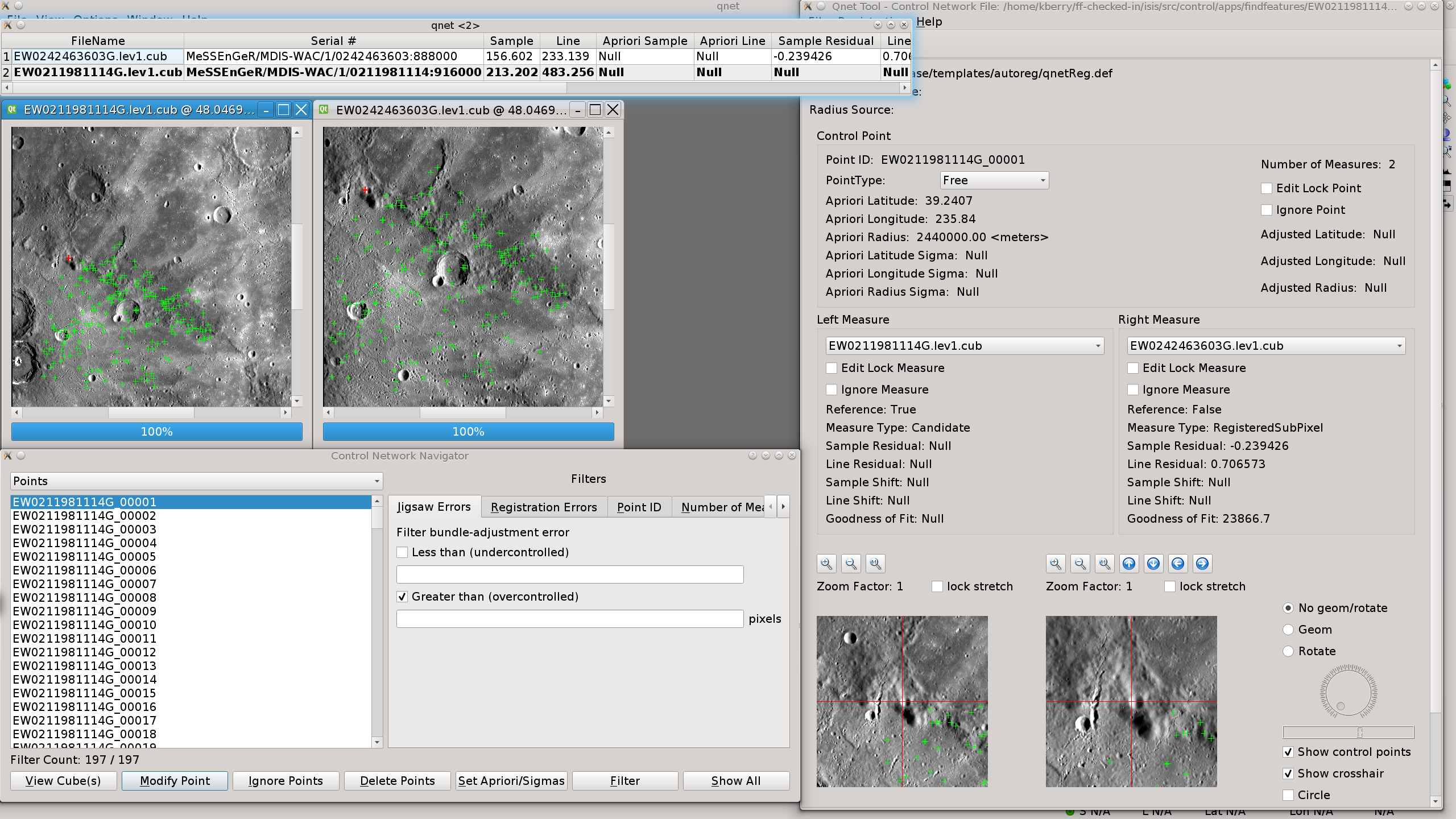
The output debug log file and a line-by-line description of the result is shown in the main application documention. And here is the screen shot of qnet for the resulting network:
Example 2
Show all the available algorithms and their default parameters
findfeatures listall=yes
Object = Algorithms
  Object = Algorithm
    CVVersion    = 4.5.5
    Name         = AGAST
    Type         = Feature2D
    Features     = Detector
    Description  = "The OpenCV AGAST Feature2D detector/extractor algorithm.
                    See the documentation at
                    http://docs.opencv.org/3.1.0/d7/d19/classcv_1_1AgastFeatur-
                    eDetector.html"
    CreatedUsing = agast
    Aliases      = (agast, detector.agast)

    Group = Parameters
      NonmaxSuppression = Yes
      Threshold         = 10
      Type              = OAST_9_16
    End_Group
  End_Object

  Object = Algorithm
    CVVersion    = 4.5.5
    Name         = AKAZE
    Type         = Feature2D
    Features     = (Detector, Extractor)
    Description  = "The OpenCV AKAZE Feature2D detector/extractor algorithm.
                    See the documentation at
                    http://docs.opencv.org/3.1.0/d8/d30/classcv_1_1AKAZE.html"
    CreatedUsing = akaze
    Aliases      = (akaze, detector.akaze, extractor.akaze, feature2d.akaze)

    Group = Parameters
      DescriptorChannels = 3
      DescriptorSize     = 0
      DescriptorType     = DESCRIPTOR_MLDB
      Diffusivity        = DIFF_PM_G2
      NOctaveLayers      = 4
      NOctaves           = 4
      Threshold          = 0.0010000000474975
    End_Group
  End_Object

  Object = Algorithm
    CVVersion    = 4.5.5
    Name         = Blob
    Type         = Feature2D
    Features     = Detector
    Description  = "The OpenCV simple blob detection algorithm. See the
                    documentation at
                    http://docs.opencv.org/3.1.0/d0/d7a/classcv_1_1SimpleBlobD-
                    etector.html"
    CreatedUsing = blob
    Aliases      = (blob, detector.blob)

    Group = Parameters
      BlobColor           = 0
      FilterByArea        = true
      FilterByCircularity = false
      FilterByColor       = true
      FilterByConvexity   = true
      FilterByInertia     = true
      MaxArea             = 5000
      maxCircularity      = inf
      MaxConvexity        = inf
      MaxInertiaRatio     = inf
      MaxThreshold        = 220
      MinArea             = 25
      MinCircularity      = 0.8
      MinConvexity        = 0.95
      MinDistance         = 10
      MinInertiaRatio     = 0.1
      MinRepeatability    = 2
      MinThreshold        = 50
      ThresholdStep       = 10
    End_Group
  End_Object

  Object = Algorithm
    CVVersion    = 4.5.5
    Name         = BRISK
    Type         = Feature2D
    Features     = (Detector, Extractor)
    Description  = "The OpenCV BRISK Feature2D detector/extractor algorithm.
                    See the documentation at
                    http://docs.opencv.org/3.1.0/de/dbf/classcv_1_1BRISK.html"
    CreatedUsing = brisk
    Aliases      = (brisk, detector.brisk, extractor.brisk, feature2d.brisk)

    Group = Parameters
      NOctaves     = 3
      PatternScale = 1.0
      Threshold    = 30
    End_Group
  End_Object

  Object = Algorithm
    CVVersion    = 4.5.5
    Name         = FAST
    Type         = Feature2D
    Features     = Detector
    Description  = "The OpenCV FAST Feature2D detector/extractor algorithm.
                    See the documentation at
                    http://docs.opencv.org/3.1.0/df/d74/classcv_1_1FASTFeature-
                    Detector.html"
    CreatedUsing = fast
    Aliases      = (detector.fast, fast, fastx)

    Group = Parameters
      NonmaxSuppression = Yes
      Threshold         = 10
      Type              = TYPE_9_16
    End_Group
  End_Object

  Object = Algorithm
    CVVersion    = 4.5.5
    Name         = GFTT
    Type         = Feature2D
    Features     = Detector
    Description  = "The OpenCV GFTT Feature2D detector/extractor algorithm.
                    See the documentation at
                    http://docs.opencv.org/3.1.0/df/d21/classcv_1_1GFTTDetecto-
                    r.html"
    CreatedUsing = gftt
    Aliases      = (detector.gftt, gftt)

    Group = Parameters
      BlockSize      = 3
      HarrisDetector = No
      K              = 0.04
      MaxFeatures    = 1000
      MinDistance    = 1.0
      QualityLevel   = 0.01
    End_Group
  End_Object

  Object = Algorithm
    CVVersion    = 4.5.5
    Name         = KAZE
    Type         = Feature2D
    Features     = (Detector, Extractor)
    Description  = "The OpenCV KAZE Feature2D detector/extractor algorithm.
                    See the documentation at
                    http://docs.opencv.org/3.1.0/d3/d61/classcv_1_1KAZE.html"
    CreatedUsing = kaze
    Aliases      = (detector.kaze, extractor.kaze, feature2d.kaze, kaze)

    Group = Parameters
      Diffusivity   = DIFF_PM_G2
      Extended      = No
      NOctaveLayers = 4
      NOctaves      = 4
      Threshold     = 0.0010000000474975
      Upright       = No
    End_Group
  End_Object

  Object = Algorithm
    CVVersion    = 4.5.5
    Name         = MSD
    Type         = Feature2D
    Features     = Detector
    Description  = "The OpenCV MSD Feature2D detector/extractor algorithm. See
                    the documentation at
                    http://docs.opencv.org/3.1.0/d6/d36/classcv_1_1xfeatures2d-
                    _1_1MSD.html"
    CreatedUsing = msd
    Aliases      = (detector.msd, msd)

    Group = Parameters
      ComputeOrientation = false
      KNN                = 4
      NMSRadius          = 5
      NMSScaleRadius     = 0
      NScales            = -1
      PatchRadius        = 3
      ScaleFactor        = 1.25
      SearchAreaRadius   = 5
      THSaliency         = 250.0
    End_Group
  End_Object

  Object = Algorithm
    CVVersion    = 4.5.5
    Name         = MSER
    Type         = Feature2D
    Features     = Detector
    Description  = "The OpenCV MSER Feature2D detector/extractor algorithm.
                    See the documentation at
                    http://docs.opencv.org/3.1.0/d3/d28/classcv_1_1MSER.html"
    CreatedUsing = mser
    Aliases      = (detector.mser, mser)

    Group = Parameters
      AreaThreshold = 1.01
      Delta         = 5
      EdgeBlurSize  = 5
      MaxArea       = 14400
      MaxEvolution  = 200
      MaxVariation  = 0.25
      MinArea       = 60
      MinDiversity  = 0.2
      MinMargin     = 0.003
    End_Group
  End_Object

  Object = Algorithm
    CVVersion    = 4.5.5
    Name         = ORB
    Type         = Feature2D
    Features     = (Detector, Extractor)
    Description  = "The OpenCV ORB Feature2D detector/extractor algorithm. See
                    the documentation at
                    http://docs.opencv.org/3.1.0/db/d95/classcv_1_1ORB.html"
    CreatedUsing = orb
    Aliases      = (detector.orb, extractor.orb, feature2d.orb, orb)

    Group = Parameters
      edgeThreshold = 31
      fastThreshold = 20
      firstLevel    = 0
      nfeatures     = 500
      nlevels       = 8
      patchSize     = 31
      scaleFactor   = 1.2000000476837
      scoreType     = HARRIS_SCORE
      WTA_K         = 2
    End_Group
  End_Object

  Object = Algorithm
    CVVersion    = 4.5.5
    Name         = SIFT
    Type         = Feature2D
    Features     = (Detector, Extractor)
    Description  = "The OpenCV SIFT Feature2D detector/extractor algorithm.
                    See the documentation at
                    http://docs.opencv.org/3.1.0/d5/d3c/classcv_1_1xfeatures2d-
                    _1_1SIFT.html"
    CreatedUsing = sift
    Aliases      = (detector.sift, extractor.sift, feature2d.sift, sift)

    Group = Parameters
      constrastThreshold = 0.04
      edgeThreshold      = 10
      nfeatures          = 0
      nOctaveLayers      = 3
      sigma              = 1.6
    End_Group
  End_Object

  Object = Algorithm
    CVVersion    = 4.5.5
    Name         = Star
    Type         = Feature2D
    Features     = Detector
    Description  = "The OpenCV Star Feature2D detector/extractor algorithm.
                    See the documentation at
                    http://docs.opencv.org/3.1.0/d6/d36/classcv_1_1xfeatures2d-
                    _1_1Star.html"
    CreatedUsing = star
    Aliases      = (detector.star, star)

    Group = Parameters
      LineThresholdBinarized = 8
      LineThresholdProjected = 10
      MaxSize                = 45
      ResponseThreshold      = 30
      SuppressNonmaxSize     = 5
    End_Group
  End_Object

  Object = Algorithm
    CVVersion    = 4.5.5
    Name         = Brief
    Type         = Feature2D
    Features     = Extractor
    Description  = "The OpenCV simple blob detection algorithm. See the
                    documentation at
                    http://docs.opencv.org/3.1.0/d0/d7a/classcv_1_1SimpleBlobD-
                    etector.html"
    CreatedUsing = brief
    Aliases      = (brief, extractor.brief)

    Group = Parameters
      Bytes          = 32
      UseOrientation = true
    End_Group
  End_Object

  Object = Algorithm
    CVVersion    = 4.5.5
    Name         = DAISY
    Type         = Feature2D
    Features     = Extractor
    Description  = "The OpenCV DAISY Feature2D detector/extractor algorithm.
                    See the documentation at
                    http://docs.opencv.org/3.1.0/d9/d37/classcv_1_1xfeatures2d-
                    _1_1DAISY.html"
    CreatedUsing = daisy
    Aliases      = (daisy, extractor.daisy)

    Group = Parameters
      H               = "1,0,0,0,1,0,0,0,1"
      interpolation   = true
      norm            = NRM_NONE
      q_hist          = 8
      q_radius        = 3
      q_theta         = 8
      radius          = 15
      use_orientation = false
    End_Group
  End_Object

  Object = Algorithm
    CVVersion    = 4.5.5
    Name         = FREAK
    Type         = Feature2D
    Features     = Extractor
    Description  = "The OpenCV FREAK Feature2D detector/extractor algorithm.
                    See the documentation at
                    http://docs.opencv.org/3.1.0/df/db4/classcv_1_1xfeatures2d-
                    _1_1FREAK.html"
    CreatedUsing = freak
    Aliases      = (extractor.freak, freak)

    Group = Parameters
      NOctaves              = 4
      OrientationNormalized = true
      PatternScale          = 22.0
      ScaleNormalized       = true
      SelectedPairs         = Null
    End_Group
  End_Object

  Object = Algorithm
    CVVersion    = 4.5.5
    Name         = LATCH
    Type         = Feature2D
    Features     = Extractor
    Description  = "The OpenCV LATCH Feature2D detector/extractor algorithm.
                    See the documentation at
                    http://docs.opencv.org/3.1.0/d6/d36/classcv_1_1xfeatures2d-
                    _1_1LATCH.html"
    CreatedUsing = latch
    Aliases      = (extractor.latch, latch)

    Group = Parameters
      Bytes              = 32
      HalfSSDSize        = 3
      RotationInvariance = true
    End_Group
  End_Object

  Object = Algorithm
    CVVersion    = 4.5.5
    Name         = LUCID
    Type         = Feature2D
    Features     = Extractor
    Description  = "The OpenCV LUCID Feature2D detector/extractor algorithm.
                    See the documentation at
                    http://docs.opencv.org/3.1.0/d6/d36/classcv_1_1xfeatures2d-
                    _1_1LUCID.html"
    CreatedUsing = lucid
    Aliases      = (extractor.lucid, lucid)

    Group = Parameters
      BlurKernel  = 1
      LucidKernel = 1
    End_Group
  End_Object

  Object = Algorithm
    CVVersion    = 4.5.5
    Name         = BFMatcher
    Type         = DecriptorMatcher
    Features     = Matcher
    Description  = "The OpenCV BFMatcher DescriptorMatcher matcher algorithm.
                    See the documentation at
                    http://docs.opencv.org/3.1.0/d3/da1/classcv_1_1BFMatcher.h-
                    tml"
    CreatedUsing = bfmatcher
    Aliases      = (bfmatcher, matcher.bfmatcher)

    Group = Parameters
      CrossCheck = No
      NormType   = NORM_L2
    End_Group
  End_Object

  Object = Algorithm
    CVVersion    = 4.5.5
    Name         = FlannBasedMatcher
    Type         = DecriptorMatcher
    Features     = Matcher
    Description  = "The OpenCV FlannBasedMatcher DescriptorMatcher matcher
                    algorithm. See the documentation at
                    http://docs.opencv.org/3.1.0/dc/de2/classcv_1_1FlannBasedM-
                    atcher.html"
    CreatedUsing = flannbasedmatcher
    Aliases      = (flannbasedmatcher, matcher.flannbasedmatcher)

    Group = Parameters
      Checks  = 32
      Epsilon = 0.0
      Sorted  = Yes
    End_Group
  End_Object
End_Object
End
Example 3
Process three images using the default radial FASTGEOM option
This example is a variation of example 1 that runs the images in a different way. This example uses the FASTGEOM option with the default settings applied to the same images. There is an additional image included that has no overlap with the MATCH image. When FASTGEOM is used, all images that cannot be mapped using ISIS geometry are excluded from the matching process. If a filename is provided in TONOGEOM option, images that do not have any common mapping points generated by the FASTGEOM pattern algorithm are written/recorded in this file. Images that are included in the matching process but do not have any control measures in common with the MATCH image will be recorded in the TONOTMATCHED filename if given.
The following command was used to create the control network of the same two images, excluding the non-overlapping image, as was processed in example 1:
findfeatures algorithm='fastx@threshold:25@type:2/brief/parameters@maxpoints:500' \
             match=EW0211981114G.cub \
             fromlist=fromlist.lis \
             fastgeom=true \
             geomtype=camera \
             geomsource=both \
             fastgeompoints=25 \
             epitolerance=3.0 \
             ratio=0.99 \
             hmgtolerance=3.0 \
             globals='FastGeomDumpMapping:true@SaveRenderedImages:true' \
             networkid="EW0211981114G_EW0242463603G" \
             pointid='EW211981116G_????' \
             onet=EW0211981114G.net \
             tolist=EW0211981114G_cubes.lis \
             tonotmatched=EW0211981114G_notmatched.lis \
             tonogeom=EW0211981114G_nogeom.lis \
             description='Create image-image control network' \
             debug=true \
             debuglog=EW0211981114G.debug.log
In this case, since we are matching more than one file, all the files to be matched must be listed, one per line, in the file specified in the FROMFILE, fromlist.lis. Here is the contents of this file:
EW0242463603G.cub
EW0218118239G.cub
There are two additional parameters added in GLOBALS parameter. The parameter FastGeomDumpMapping:true will notify the radial mapping algorithm to dump a CSV file containing the results of the common mapping points generated from the radial pattern. Recall that the radial algorithm produces only one pattern from which it calculates the perspective warping matrix for each image in the FROMLIST. This option generates a file containing the data made up of the basenames of the MATCH and FROMLIST image pairs. In this example, the file EW0211981114G_EW0242463603G.radial.fastgeom.csv is created. Even files that cannot be mapped will have a file generated but they will be empty. This matrix is then applied to the FROMLIST image that is intended to better correspond spatially with the MATCH image. The SaveRenderedImages:true parameter tells findfeatures to save the warped images to a PNG file. This will allow users to evaluate how well the FASTGEOM algorithm performed. This option creates PNG files generated from their base file names, such as EW0211981114G_query.png from the MATCH file and EW0242463603G_train.png from the FROMLIST file name. The processing of FASTGEOM is logged in the DEBUGLOG file if given and DEBUG=true is set. Here is the portion of the log file EW0211981114G.debug.log that is created from the FASTGEOM algorithm:
---------------------------------------------------
Program:        findfeatures
Version         1.2
Revision:       2023-06-16
RunTime:        2023-06-19T11:44:03
OpenCV_Version: 4.5.5

System Environment...
Number available CPUs:     8
Number default threads:    8
Total threads:             8

Image load started at  2023-06-19T11:44:03

++++ Running FastGeom ++++
*** QueryImage: EW0211981114G.cub
*** TrainImage: EW0242463603G.cub
  FastGeomAlgorithm:            radial
  FastGeomPoints:               25
  FastGeomTolerance:            3
  FastGeomQuerySampleTolerance: 0
  FastGeomQueryLineTolerance:   0
  FastGeomTrainSampleTolerance: 0
  FastGeomTrainLineTolerance:   0

--> Using Radial Algorithm train-to-query mapping <--
  FastGeomMaximumRadius:         724.077
  FastGeomRadialSegmentLength:   25
  FastGeomRadialPointCount:      5
  FastGeomRadialPointFactor:     1
  FastGeomRadialSegments:        29

==> Radial Point Mapping complete <==
  TotalPoints:     2031
  ImagePoints:     1333
  MappedPoints:    1333
  InTrainMapFOV:   636

--> Dumping radial points <---
  PointDumpFile:     EW0211981114G_EW0242463603G.radial.fastgeom.csv
  TotalPoints:       1333

==> Geometric Correspondence Mapping complete <==
  TotalPoints:       636

--> Running Homography Image Transform <---
  IntialPoints:       636
  Tolerance:          3
  TotalLmedsInliers:  563
  PercentPassing: 88.522

  MatrixTransform:
    0.645981,-0.0158572,113.771
    -0.0350108,0.628872,337.353
    -8.52086e-05,2.53351e-06,1


++++ Running FastGeom ++++
*** QueryImage: EW0211981114G.cub
*** TrainImage: EW0218118239G.cub
  FastGeomAlgorithm:            radial
  FastGeomPoints:               25
  FastGeomTolerance:            3
  FastGeomQuerySampleTolerance: 0
  FastGeomQueryLineTolerance:   0
  FastGeomTrainSampleTolerance: 0
  FastGeomTrainLineTolerance:   0

--> Using Radial Algorithm train-to-query mapping <--
  FastGeomMaximumRadius:         724.077
  FastGeomRadialSegmentLength:   25
  FastGeomRadialPointCount:      5
  FastGeomRadialPointFactor:     1
  FastGeomRadialSegments:        29

==> Radial Point Mapping complete <==
  TotalPoints:     2031
  ImagePoints:     1333
  MappedPoints:    0
  InTrainMapFOV:   0

--> Dumping radial points <---
  PointDumpFile:     EW0211981114G_EW0218118239G.radial.fastgeom.csv
  TotalPoints:       0

==> Geometric Correspondence Mapping complete <==
  TotalPoints:       0
>>>> ERROR - Failed to get FOV geometry mapping for EW0218118239G.cub to EW0211981114G.cub needing 25 but got 0 in train FOV.
Failed to load EW0218118239G.cub

Image load complete at 2023-06-19T11:44:04

Total failed image loads/FastGeoms excluded: 1
EW0218118239G.cub

See also EW0211981114G_nogeom.lis

Total Algorithms to Run:     1

@@ matcher-pair started on 2023-06-19T11:44:04
Note that an error is shown for the file EW0218118239G.cub. This is because no common points were found for this file and the MATCH file, EW0211981114G. Using the "keyword:value" pairs in the GLOBALS parameters, the results can be analyzed as shown in the panel below. The plot in the lower left corner of the panel shows the results of the FASTGEOM Radial parameter geometry mapping of common/cooresponding points of the MATCH and FROM image. The points in red are outside the FROM image FOV and do not contribute to the computation of the homography matrix for the perspective warp for spatial consistency with the MATCH image. The blue points are the ones used in to produce the homography matrix. The image in the lower right corner is the result of the warp of the FROM image.
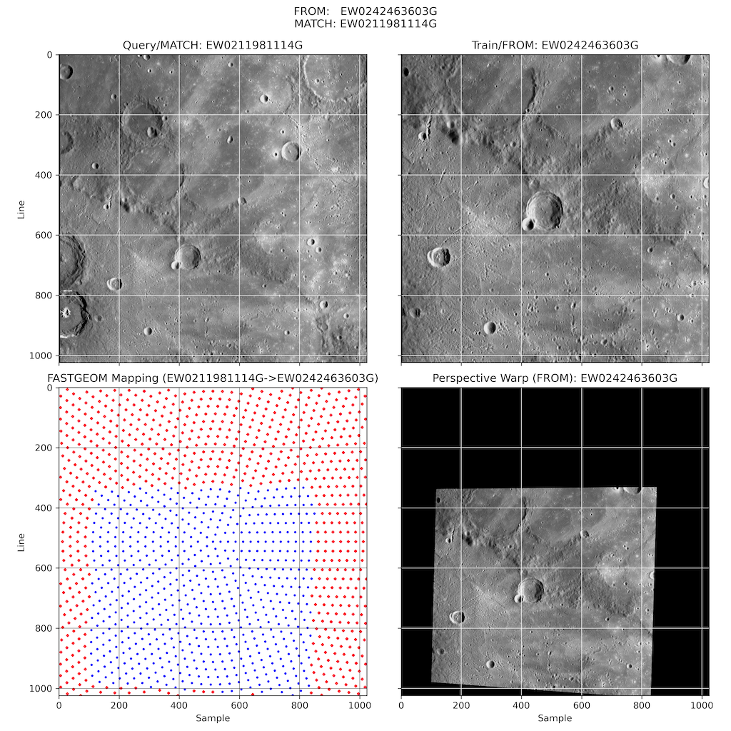
The network produced from this example contains 145 control points and with two measures each (290). This screen shot shows the resulting network. The pointreg application should be run on this network to refine the control measures to sub-pixel accuracy.
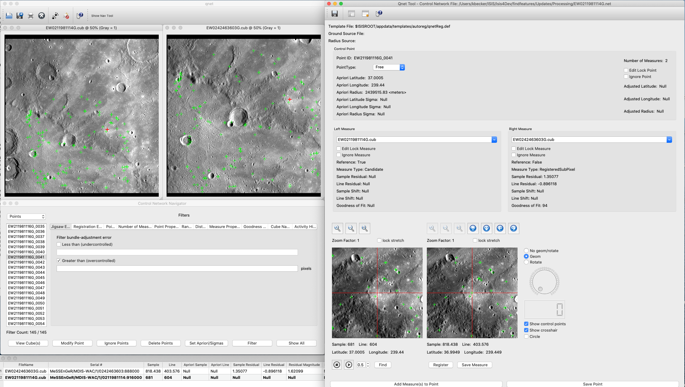
Example 4
Create a controlled mosaic using findfeatures
Overview
This example shows the results of a comprehensive processing sequence that produces a controlled mosaic using findfeatures. The data used for this mosaic is MESSENGER MDIS NAC and WAC EDR images of Mercury taken from the MESSENGER MDIS PDS archive. These EDRs are ingested into ISIS and standard processing is then applied producing the regional controlled mosaic using findfeatures. The EDR images used for this example are:
EN0108828436M.IMG
EN0108828483M.IMG
EN0108828488M.IMG
EN0217733143M.IMG
EN0217733334M.IMG
EN0218118182M.IMG
EW0215590428G.IMG
EW0218075871G.IMG
EW0218118239G.IMG
It is important to recognize the procedures applied here are effective under limited conditions. Namely, all the images included here have some common overlap with the carefully chosen MATCH image. Adding additional images that do not overlap the MATCH image will be excluded by findfeatures and requires additional steps that utilize techniques outside the scope of this example. It would involve repeatedly running findfeatures where every image is used as the MATCH image and all other images are included in the FROMLIST (with common ground coverage) and the resulting image-based networks are combined into a single network. This technique is also used for larger, global networks that frequently have images with largely varying resolutions and observing conditions. This technique has successfully been used to create global networks for Mercury using MESSENGER MDIS images and Bennu using OSIRIS-REx OCAMS images.
Making a Controlled Mosaic with findfeatures
The MESSENGER NAC and WAC images must be processed with the ISIS application processing sequence of mdis2isis, spiceinit, mdiscal, camstats and footprintinit. This will prepare the images for findfeatures which will create an image-based network. The findfeatures command used on these nine images which performs image matching and creates the network is:
base="EW0218118239G"
findfeatures algorithm='fastx@threshold:25@type:2/brief/parameters@Maxpoints:7000' \
             match="${base}.cal.cub" \
             fromlist=fromlist.lis \
             fastgeom=true \
             geomtype=camera \
             geomsource=both \
             fastgeompoints=50 \
             epitolerance=7.0 \
             ratio=0.99 \
             hmgtolerance=7.0 \
             globals='FastGeomDumpMapping:true@SaveRenderedImages:true@FastGeomAlgorithm:grid' \
             networkid="${base}_Mosiac" \
             pointid="${base}_????" \
             onet="${base}.net" \
             tolist="${base}_cubes.lis" \
             tonotmatched="${base}_notmatched.lis" \
             tonogeom="${base}_nogeom.lis" \
             description='Create MESSENGER MDIS image-image control network' \
             debug=true \
             debuglog="${base}.debug.log"
There are several things to note. The maximum number of points to retain from each image is limited in the detector (7000) as specified in the "/parameter" section of the algorithm specification. The fastx detector will very frequently produce a significant number of keypoints. This may seem like a lot of keypoints per image pair, but is likely a good choice for some images sets that contain different pixel resolutions or largely varying observation conditions like what is seen in this dataset. We are using the FASTGEOM Grid algorithm (specified in the GLOBALS program option) because the default Radial will have a difficult time meeting the minimum number of FASTGEOMPOINTS points due to large variations in pixel resolutions. The transformed files are retained so the FASTGEOM performance can be evaluated. The HMGTOLERANCE and EPITOLERANCE are both set to 7 pixels to account for uncertainty in SPICE data and distortions in the translated images due to the linear nature of the perspective warp transform caused by topography differences (which should be accounted for in an ensuing run of pointreg in the definition file by setting the size of the SearchChip to be larger that twice the size of the tolerances). We expect no files in the TONOGEOM and TONOTMATCHED because no such problems exist in this example. And you should have a look at the output DEBUGLOG file for detailed performance and behavior information for findfeatures that may indicate the need for adjustments of the matching parameters.
The MATCH image, EW0218118239G, was carefully chosen in this dataset because it has common ground coverage/overlap with all the other eight MDIS images. qmos is most helpful to determine this image as a MATCH candidate as is shown in this screen shot. Image EW0218118239G is the one outlined with the dashed square. It is clear there are images with largely varying pixel resolutions. Users will be able to select any image by changing the "base" variable in prior to the execution of findfeatures.
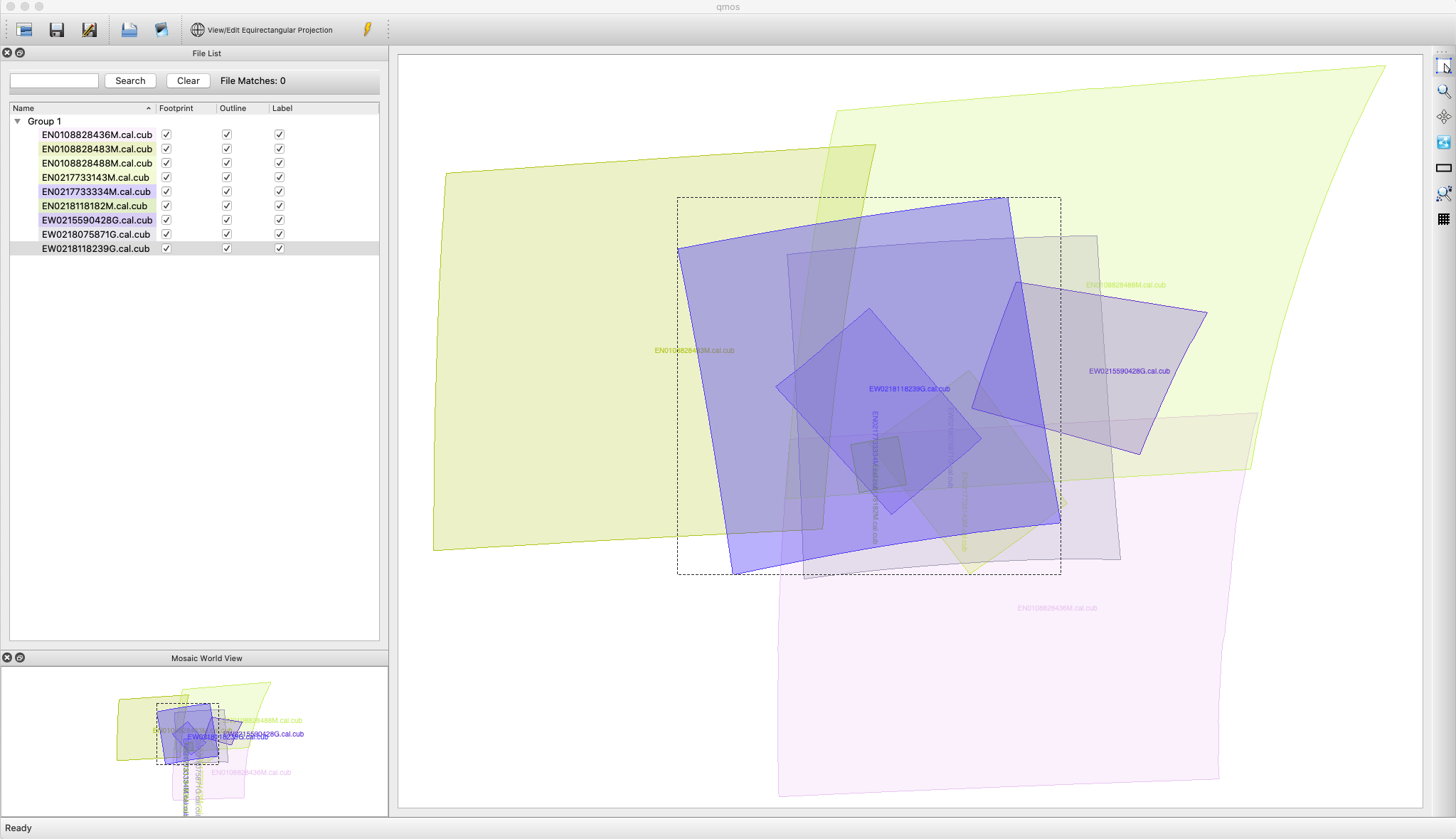
The control network created by findfeatures is an image-based network. This type of network will contain no points outside the FOV of the MATCH image. In most cases when building a larger network, a single image-based network is insufficient to produce a large connected network, so successive runs of findfeatures using different MATCH files is required. This image-based network contains 3940 control points. The best networks will have the deepest control points (i.e., contains many measures that includes all images matched). Typically this is not realistic so additional options can be considered. For example, success in jigsaw is greatly increased by the quality of the control points/measures. The pointreg application is used to refine control measures in the output network produced by findfeatures to sub-pixel accuracy. This step is where this result can be achieved by setting a high Tolerance in the Algorithm group of the REGDEF file. For great control points, use Tolerance = 0.9, which is what was used in this example. The network produced by findfeatures initially resulted in 4646 control points with 12,203 control measures with a maximum of 7 control measures in a control point. However, the average number of measures was 2.6, which indicates the majority of control points contain 2-3 measures - not so great. However, looking carefully at the qmos data, there is not much potential for deeper control points because of limited overlapping images. To increase this number you can further increase HMGTOLERANCE and EPITOLERANCE, or choose a different set of matching algorithms. After pointreg, 3940 control points with 8338 control measures remain, an average of 2.116 measures/point. This is pretty good considering how high the Tolerance was set. The other thing to consider is the distribution of the points. The screen shot below shows the point distribution and density for each image. Given the minimum coverage of many of the images, this will work - or at least be worth producing a mosaic for evaluation.
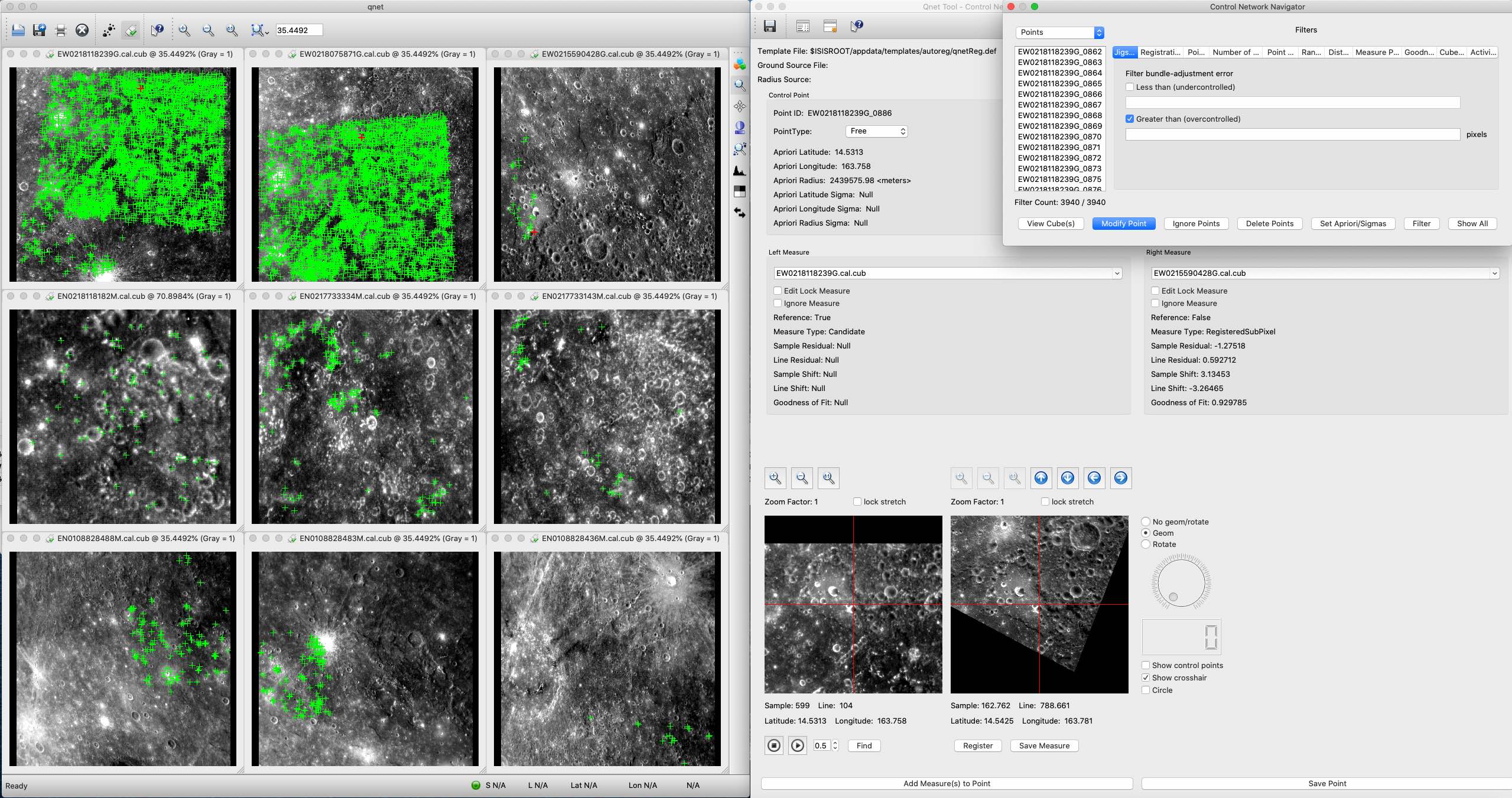
Producing a mosaic is the best way to assess the quality of the network. It is recommended to create both an uncontrolled and controlled mosaic to visually inspect/compare with qview or an alternative image viewer. The screen shot below shows a portion of the two mosaics. One important thing to note is this example does not control to a ground truth source. There are at least several ways to control your mosaic to ground truth but that is outside the scope of this example (and they are typically a great deal of work!). With that said, the spacecraft position serves as our "ground truth" but you may also see the MATCH image will have the least adjustment because it is highly biased since it has the most control measures.