Overview
The jigsaw application performs a photogrammetric bundle adjustment on a group of
overlapping, level 1 cubes from framing and/or line-scan cameras. The adjustment
simultaneously refines the selected image geometry information (camera pointing, spacecraft
position) and control point coordinates (x,y,z or lat,lon,radius) to reduce
boundary mismatches in mosaics of the images.
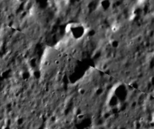
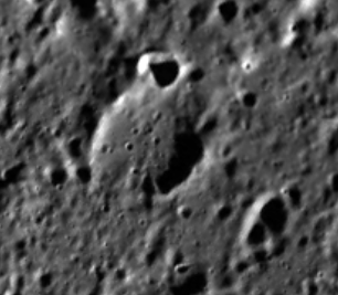
This functionality is demonstrated below in a zoomed-in area of a mosaic of a
pair of overlapping Messenger images. In the before jigsaw mosaic on the left
(uncontrolled), the features on the edges of the images do not match. In the after
jigsaw mosaic on the right (controlled), the crater edges meet correctly and the
seam between the two images is no longer visible.


The jigsaw application assumes spiceinit or csminit has been run on the
input cubes so that camera information is included in the Isis cube
labels. In order to run the program, the user must provide a list of input cubes,
an input control net, the name of an output control network, and the
solve settings. The measured sample/line positions associated with the
control measures in the network are not changed. Instead, the control points and
camera information are adjusted. jigsaw outputs a new control network that
includes the initial state of the points in the network and their final state after the
adjustment. The initial states of the points are tagged as a priori in the
control network, and their final states are tagged as adjusted.
Updated camera information is only written to the cube labels if the bundle
converges and the UPDATE parameter is selected.
In order to apply bundle values using ADJUSTMENT_INPUT, only the option FROMLIST
must be set. If the ADJUSTMENT_INPUT is set to an HDF5 file containing bundle adjustment values
(usually the HDF5 output file from OUTADJUSTMENTH5), those values can be applied to the
cube labels. The adjustment file entails a group of HDF5 datasets where each dataset
contains the instrument pointing and position for each cube. The dataset key is composed
of the cube serial number and the table name, either "InstrumentPointing" or
"InstrumentPosition", separated by a forward slash "/". For example:
      SerialNumber: MRO/CTX/1016816309:030
      Dataset key for instrument pointing: MRO/CTX/1016816309:030/InstrumentPointing
The input control net may be created by finding each image footprint with footprintinit,
computing the image overlaps with findimageoverlaps, creating guess measurements with
autoseed, then registering them with pointreg.
Optional output files can be enabled to provide more information for analyzing the results of
the bundle. BUNDLEOUT_TXT provides an overall summary of the bundle adjustment;
it lists the user input parameters selected and tables of statistics for both the
images and the points. The image statistics can be written to a separate machine readable
file with the IMAGESCSV option and likewise for the point statistics with the
OUTPUT_CSV option. RESIDUALS_CSV provides a table of the measured image
coordinates, the final sample, line, and overall residuals
of every control measure in both millimeters and pixels. OUTADJUSTMENTH5 stores bundle
adjustment values in an HDF5 file. Currently, only ISIS adjustment values are saved to file so
if all the cubes in the FROMLIST contain a CSM state blob then the adjustment_out.h5
file will be created but empty.
Observation Equations
The jigsaw application attempts to minimize the reprojective error within the control network.
For each control measure and its control point in the control network, the reprojective error is
the difference between the control measure's image coordinate (typically determined from image
registration)
and the image coordinate that the control point projects to through the camera model. We also
refer to the reprojective error as the measure residual. So, for each control measure we can
write an observation equation:
reprojective_error = control_measure - camera(control_point)
The camera models use additional parameters such as the instrument position and pointing to compute
what image coordinate a control point projects to; so, the camera function in our observation
equation can be written more explicitly as:
reprojective_error = control_measure - camera(control_point, camera_parameters)
The primary decision when using the jigsaw application is which parameters to include
as variables in the observation equations. Later sections will cover what parameters can
be included and common considerations when choosing them.
By combining all the observation equations for all the control measures in the control network
we can create a system of equations. Then, we can find the camera parameters and control point
coordinates that minimize the sum of the squared reprojective errors using the system of equations.
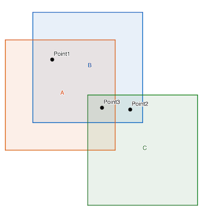
Below is an example system of observation equations for a control network with three images
(A, B, and C) and three control points (1, 2, and 3). Control point 1 has control measures
on images A and B, control point 2 has control measures on images B and C, and control
point 3 has control measures on images A, B, and C. control_point_1 is the
ground coordinate of control point 1, camera_parameters_A are the camera
parameters for image A's camera model, camera_A is the projection function
for image A's camera model, and control_measure_1_A is the image coordinate of
control point 1's control measure on image A.

                    || control_measure_1_A - camera_A(control_point_1, camera_parameters_A) ||
                    || control_measure_1_B - camera_B(control_point_1, camera_parameters_B) ||
                    || control_measure_2_B - camera_B(control_point_2, camera_parameters_B) ||
      total_error = || control_measure_2_C - camera_C(control_point_3, camera_parameters_C) ||
                    || control_measure_3_A - camera_A(control_point_3, camera_parameters_A) ||
                    || control_measure_3_B - camera_B(control_point_3, camera_parameters_B) ||
                    || control_measure_3_C - camera_C(control_point_3, camera_parameters_C) ||
If the camera projection functions were linear, we could easily minimize this system. Unfortunately,
the camera projection functions are quite non-linear; so, we linearize and
iteratively compute updates that will gradually approach a minimum. The actual
structure of the observation equations is complex and vary significantly
based on the dataset and which parameters are being solved for. If the a-priori parameter
values are sufficiently far away from a minimum, the updates can even diverge. So,
it is important to check your input data set and solve options. Tools like the
cnetcheck application and jigsaw options like OUTLIER_REJECTION can help.
As with all iterative methods convergence criteria is important. The default for
the jigsaw application is to converge based on the sigma0 value. This is a
complex value that includes many technical details outside the scope of this
documentation. In a brief, it is a measurement of the remaining error in a typical
observation. The sigma0 value is also a good first estimate of the quality
of the solution. If the only errors in the control network are purely random noise,
then the sigma0 should be 1. So, if the sigma0 value for your solution is
significantly larger than 1, then it is an indication that there is an unusual
source of error in your control network such as poorly registered control measures
or poor a-priori camera parameters.
Solve Options
Choosing solve options is difficult and often requires experimentation. As a general rule,
the more variation in observation geometry in your dataset and the better distributed your
control measures are across and within images, the more parameters you can solve for.
The following sections describe the different options you can use when running the
jigsaw application. Each section will cover a subset of the options explaining
common situations in which they are used and how to choose values for them.
Control Network
Control networks can contain a wide variety of information, but the primary
concern for choosing solve options is the presence or lack of ground control.
Most control networks are generated by finding matching points between groups
of images. This defines a relative relationship between the images, but it does not
relate those images to the actual planetary surface; so, additional information is needed
to absolutely control the images. In terrestrial work, known points on the ground
are identified in the imagery via special target markers, but this is usually not
possible with planetary data. Instead, we relate the images to an additional dataset such
as a basemap or surface model. This additional relationship is called ground
control. Sometimes, there are not sufficient previous data products to provide accurate
ground control or ground will be done as a secondary step after successfully running jigsaw
on a relatively controlled network. In both these cases, we say that ground
control is not present.
If your control network does not have ground control, then we recommended that
you hold the instrument position fixed and only solve for the instrument pointing.
This is because without ground control, the instrument position and pointing can
become correlated and there will be multiple minimums for the observation equations.
We recommend holding the instrument position fixed because a-priori data for it generally is more
accurate than the instrument pointing.
Sensor Types
Framing
Framing sensors are the most basic type or sensor to use with jigsaw. The entire image is exposed at the same
time, so there is only a single position and pointing value for each image. With these datasets
you will want to use the either NONE or POSITIONS for the SPSOLVE parameter and ANGLES
for the CAMSOLVE parameter.
Pushbroom
Pushbroom sensors require additional consideration because the image is exposed over a period of
time and therefore, position and pointing are time dependent. The jigsaw application handles this
by modeling the position and pointing as polynomial functions of time. Polynomial functions
are fit to the a-priori position and pointing values on each image. Then, each iteration updates
the polynomial coefficients. Setting CAMSOLVE to velocities will use first
degree, linear, polynomials and setting CAMSOLVE to accelerations will use
second degree, quadratic, polynomials for the pointing angles. For most pushbroom observations,
we recommend using second degree polynomials, solving for accelerations.
There are also a variety of parameters that allow for more precise control over the polynomials used
and the polynomial fitting process. The OVERHERMITE parameter changes the initial polynomial
setup so that it does not replace the a-priori position values. Instead, the polynomial starts out as a
zero polynomial and is added to the original position values. This effectively adds the noise
from the a-priori position values to the constant term of the polynomial. The OVEREXISTING
parameter does the same thing for pointing values. These two options allow you to preserve complex
variation like jitter. We recommend enabling these options for jittery images and very long
exposure pushbroom images.
The SPSOLVE and CAMSOLVE parameters only allow up to a second degree
polynomial. To use a higher degree polynomial for pointing values, set CAMSOLVE to ALL and then set
the CKDEGREE parameter to the degree of the polynomial you want to fit over the original
pointing values and set the CKSOLVEDEGREE parameter to the degree of the polynomial you want
to solve for. Setting the SPSOLVE, SPKDEGREE, and SPKSOLVEDEGREE parameters
in a similar fashion gives fine control over the polynomial for postion values.
For example, if you want to fit a 3rd degree polynomial for the position values
and then solve for a 5th degree polynomial set SPSOLVE to ALL, SPKDEGREE to 3,
and SPKSOLVEDEGREE to 5.
These parameters should only be used when you know the a-priori position and/or pointing values are
well modeled by high degree polynomials. Using high degree polynomials can result in extreme
over-fitting where the solution looks good in areas near control measures and control points but
is poor in areas far from control measures and control points. The end behavior, the solution at
the start and end of images, becomes particularly unstable as the degree of the polynomial used
increases.
Synthetic Aperture Radar
Running the jigsaw application with synthetic aperture radar (SAR) images is different because
SAR sensors do not have a pointing component. Thus, you can only solve for the sensor position when
working with SAR imagery. SAR imagery also tends to have long duration images which can
necessitate using the OVERHERMITE, SPKDEGREE, and SPKSOLVEDEGREE parameters.
Parameter Sigmas
The initial, or a-priori, camera parameters and control points all contain error, but it is not equally
distributed. The jigsaw application allows users to input a-priori sigmas for different parameters
that describe how the initial error is distributed. The parameter sigmas are also sometimes
called uncertainties. Parameters with higher a-priori sigma values
are allowed to vary more freely than those with lower a-priori sigma values. The a-priori sigma values
are not hard constraints that limit how much parameters can change, but rather relative accuracy estimates
that adjust how much parameters change relative to each other.
The POINT_LATITUDE_SIGMA, POINT_LONGITUDE_SIGMA, and POINT_RADIUS_SIGMA
parameters set the a-priori sigmas for control points that do not already have a ground source.
If a control point already has a ground source, such as a basemap or DEM, then it already has
internal sigma values associated with it or is held completely fixed. The exact behavior depends
on how the control points were created, a topic outside the scope of this documentation.
These sigmas are in meters on the ground, so the latitude
and longitude sigmas are uncertainty in meters in the latitude and longitude directions. Generally, you will
choose values for these parameters based on the resolution of the images and a visual comparison with
other datasets. The radius sigma is also usually higher than the latitude and longitude sigmas
because there is less variation of the viewing geometry with respect to the radius.
The CAMERA_ANGLES_SIGMA, CAMERA_ANGULAR_VELOCITY_SIGMA, and
CAMERA_ANGULAR_ACCELERATION_SIGMA parameters set the a-priori sigmas for the instrument pointing.
Similarly, the SPACECRAFT_POSITION_SIGMA, SPACECRAFT_VELOCITY_SIGMA,
and SPACECRAFT_ACCELERATION_SIGMA parameters set the a-priori sigmas for the instrument position.
The sigma for each parameter is only used if you are solving for that parameter. For example,
if you are solving for angular velocities and not solving for any adjustments to the instrument
position you would enter CAMERA_ANGLES_SIGMA and CAMERA_ANGULAR_VELOCITY_SIGMA.
Finding initial values for these sigmas is challenging as SPICE does not have a way to specify them.
Some teams will publish uncertainties for their SPK and CK solutions in separate documentation or
the kernel comments, the
commnt utility
will read the comments on a kernel file. The velocity
and acceleration sigmas are in meters per second and meters per second squared respectively
(degrees per second and degrees per second squared for angles). So, the velocity sigma will
generally be smaller than the position sigma and the acceleration sigma will be smaller than
the velocity sigma.
Coming up with a-priori sigma values can be quite challenging, but the jigsaw application
has the ability to produce updated sigma values for your solution. By enabling the ERRORPROPAGATION
parameter, you will get a-posteriori (updated) sigmas for each control point and camera parameter
in your solution. This information is helpful for analyzing and communicating the quality of
your solution. Computing the updated sigmas, imposes a significant computation and memory
overhead, so it is recommended that you enable ERRORPROPAGATION parameter after you
have run bundle adjustment with all of your other settings and gotten a satisfactory result.
Community Sensor Model
The jigsaw options that control which parameters to solve for only work with ISIS
camera models. When working with community sensor model (CSM) camera models, you will
need to manually specify the camera parameters to solve for. This is because the
CSM API only exposes a
generic camera parameter interface that may or may not be related to the physical state of the
sensor when an image was acquired. The CSMSOLVELIST option allows for an explicit list
of model parameters. You can also use the CSMSOLVESET or CSMSOLVEYPE options
to choose your parameters based on how they are labeled in the model.
Each CSM plugin library defines its own set of adjustable parameters. See the
documentation for the CSM plugin library you are using for what different adjustable parameters
are and when to solve for them. The sigma values for parameters are also included in the CSM plugin
library and image support data (ISD). So, you do not need to specify camera parameter sigmas when
working with CSM camera models; however, you still need to specify control point coordinate sigmas.
For convenience, the csminit application adds information about all of the adjustable
parameters to the image label.
The CSM API natively uses a rectangular coordinate system. So, we recommend that
you have the jigsaw application perform calculations in a rectangular coordinate system
when working with CSM camera models. To do this, set the CONTROL_POINT_COORDINATE_TYPE_BUNDLE
parameter to RECTANGULAR. You can also set the
CONTROL_POINT_COORDINATE_TYPE_REPORTS parameter to RECTANGULAR to see the
results in a rectangular coordinate system, but this is a matter of personal preference
and will not impact the results.
Robustness
Much of the mathematical underpinning of the jigsaw application expects that the error
in the input data is purely random noise. If there are issues with control measures being
poorly registered or blatantly wrong, it can produce errors in the output solution. Generally,
users should identify and correct these errors before accepting the output of the jigsaw
application, but there are a handful of parameters than can be used to make your solutions more
robust to them.
The OUTLIER_REJECTION parameter adds a simple calculation to each iteration that looks
for potential outliers. The median average deviation (MAD) of the measure residuals is computed
and then any control measure whose residual is larger than a multiple of the MAD of the measure residuals
is flagged as rejected. Control measures that are flagged as rejected are removed
from future iterations. The multiplier for the rejection threshold is set by the
REJECTION_MULTIPLIER parameter. The residuals for rejected measures are re-computed
after each iteration and if they fall back below the threshold they are un-flagged
and included again. Enabling this parameter can help eliminate egregious errors in your control
measures, but it is not very sensitive. It is also not selective about what is rejected.
So, it is possible to introduce islands into your control network when the OUTLIER_REJECTION
parameter is enabled. For this reason, always check your output
control network for islands with the cnetcheck application when using the
OUTLIER_REJECTION parameter. Choosing an appropriate value for the REJECTION_MULTIPLIER
is about deciding how aggressively you want to eliminate control measures. The default value
will only remove extreme errors, but lower values will remove control measures that are not
actually errors. It is recommended that you start with the default value and then if you want to remove
more potential outlier, reduce it gradually. If you are seeing too many rejections with the
default value, then your input data is extremely poor and you should investigate other methods
of improving it prior to running the jigsaw application. You can use the qnet
application to examine and improve your control network. You can use the qtie application
to manually adjust your a-priori camera parameters.
The jigsaw application also has the ability to set sigmas for individual control
measures. Similar to the sigmas for control points and parameters, these are a measurement
of the relative quality of each control measure. Control measures with a higher sigma have less
impact on the solution than control measures with a lower sigma. Most control networks have
a large number of control measures and it is not realistic to manually set the sigma for
each one. So, the jigsaw application can instead use maximum likelihood estimation (MLE)
to estimate the sigma for each control measure each iteration. There are a variety of models to
choose from, but all of them start each control measure's sigmas at 1. Then, if the control
measure's reprojective error falls beyond a certain quantile the sigma will be increased.
This reduces the impact of poor control measures in a more targeted fashion than simple
outlier rejection. In order to produce good results, though, a high density of control measures
is required to approximate the true reprojective error probability distributions. Some of the
modules used with MLE can set a measure's sigma to infinity, effectively removing it from the
solution. Similar to when using the OUTLIER_REJECTION parameter, this can create islands
in your control network. If you are
working with a large amount of data and want a robustness option that is more targeted and
customizable than outlier rejection, then using the MLE parameters is a good option. See the
MODEL1, MODEL2, MODEL3, MAX_MODEL1_C_QUANTILE,
MAX_MODEL2_C_QUANTILE, and MAX_MODEL3_C_QUANTILE parameter documentation for
more information.
Observation Mode
Sometimes multiple images are exposed at the same time. They could be exposed by different sensors
on the same spacecraft or they could be read out from different parts of the same sensor. When
this happens, many of the camera parameters for the two images are the same. By default, the
jigsaw application has a different set of camera parameters for each image. To allow
different images that are captured simultaneously to share camera parameters enable the
OBSERVATIONS parameter. This will combine all of the images with the same observation
number into a single set of parameters. By default the observation number for an image is the
same as the serial number. For some instruments, there is an extra keyword in their serial number
translation file called ObservationKeys. This specifies the number of keys from the
serial number to use in the observation number. For example JunoCam serial numbers consist of
SpacecraftName/InstrumentId/StartTime/FrameNumber/FilterName and it has
ObservationKeys = 4. So, the observation number for a JunoCam image is the first
four keys of its serial number, SpacecraftName/InstrumentId/StartTime/FrameNumber.
Thus, if two JunoCam images have the same StartTime and FrameNumber but different FilterNames
and the OBSERVATIONS parameter is enabled, then they will share camera parameters.
To check if observation mode
is setup for use with your data set, check the serial number translation file located in
$ISISROOT/appdata/translations.
References
For information on what the original jigsaw code was based on checkout
Rand Notebook
A more technical look at the jigsaw application can be found in
Jigsaw: The ISIS3 bundle adjustment for extraterrestrial photogrammetry
by K. L. Edmundson et al.
A rigorous development of how the jigsaw application works can be found
in these
lecture notes
from Ohio State University.
Known Issues
Running jigsaw with a control net containing JigsawRejected
flags may result in bundle failure
When running jigsaw with Outlier Rejection turned on,
control points and/or control measures may be flagged as
JigsawRejected in the output control net file. If this output net
file is then used in a subsequent jigsaw run, these points and
measures will be erroneously ignored, potentially causing the bundle
adjustment to fail.
--Workarounds
- Run jigsaw with Outlier Rejection off.
- Do not use the output control net file in subsequent jigsaw runs.
- Convert the output control net file from binary to PVL and back using
cnetbin2pvl and cnetpvl2bin. This will
clear the JigsawRejected flags.
Solving for the target body radii (triaxial or mean) is NOT possible and
likely increases error in the solve.
With the current jigsaw implementation, it is NOT possible to individually
solve for either the mean or triaxial radii as separate calculations in
the bundle adjustment. More specifically, the target body radii have no
effect when solving for individual points and thus cannot be solved for in the bundle.
A local radii solve is already part of the sequence of equations that jigsaw
uses to compute various partial derivatives to populate the solve matrix.
A separate mean or triaxial radii solve can be applied to the target body
and the partials from this separate application are added to the
solve matrix. This option adds additional computation time to jigsaw
and creates additional uncertainty/error in the bundle adjust. We advise
the mean and triaxial radii solve be avoided.
If you are trying to generate a spheroid from a control network there are
other programs that can do this for you. An easier but more naive method
is ingesting the OUTPUT_CSV from your network, gather local radii
information from those points, then generate a spheroid from those local radii.
| Jeff Anderson | 2007-04-27 |
Original version
|
| Steven Lambright | 2007-07-23 |
Changed category to Control Networks and corrected XML bugs
|
| Debbie A. Cook | 2007-10-05 |
Revised iteration report to list the errors and sigmas from the same iteration. Previous
version reported errors from previous iteration and sigmas from current iteration.
|
| Christopher Austin | 2008-07-03 |
Cleaned the Bundle Adjust memory leak and fixed the app tests.
|
| Tracie Sucharski | 2009-04-08 |
Added date to the Jigged comment in the spice tables.
|
| Tracie Sucharski | 2009-04-22 |
If updating pointing, delete the CameraStatistics table from labels.
|
| Mackenzie Boyd | 2009-07-23 |
Modified program to write history to input cubes.
|
| Debbie A. Cook | 2010-08-12 |
Commented out Heldlist until mechanism in place to enter individual
image parameter constraints.
|
| Debbie A. Cook | 2010-08-12 |
Merged Ken Edmundson version with system and binary control net.
|
| Debbie A. Cook | 2011-06-14 |
Modified code to prevent updates to cube files in held list.
|
| Debbie A. Cook | 2011-09-28 |
Removed SC_SIGMAS from user parameter list because it is not
fully implemented; changed method name SPARSE to OLDSPARSE
and CHOLMOD to SPARSE; and improved the documentation for
the Isis3.3.0 release.
|
| Debbie A. Cook, Ken Edmundson, and Orrin Thomas | 2011-10-03 |
Added images showing before and after to demonstrate the
program. Added Krause's collinearity diagram and
a brief explanation on the output options. Also added
a lien for example(s) to be added later.
|
| Debbie A. Cook | 2011-10-06 |
Corrected previous history entry and added references to glossary. Also
changed application names to bold type.
|
| Debbie A. Cook and Ken Edmundson | 2011-10-07 |
Removed glossary references from briefs. Also changed the definition
of angles to state right ascension and declination to be consistent
with the output.
|
| Ken Edmundson | 2011-10-14 |
Added internal default and minimum inclusive tags to global apriori
uncertainties.
|
| Ken Edmundson | 2011-10-18 |
Added Known Issues section and JigsawRejected flag issue.
|
| Debbie A. Cook | 2011-11-04 |
Added minimums to parameters, corrected SOLVEDEGREE description, and
added to the camsolve option descriptions in response to Mantis
issue #514.
|
| Ken Edmundson | 2011-12-20 |
Added REJECTION_MULTIPLIER to interface, part of Mantis issue #637.
|
| Ken Edmundson | 2012-01-19 |
Added SPKDEGREE and SPKSOLVEDEGREE; changed name of SOLVEDEGREE to
CKSOLVEDEGREE.
|
| Ken Edmundson | 2014-02-13 |
Added separate group for Error Propagation with option to write inverse matrix to binary
file. For extremely large networks where memory/time for error propagation is limited.
|
| Ken Edmundson | 2014-07-09 |
Added USEPVL and SC_PARAMETERS parameters.
|
| Jeannie Backer | 2014-07-14 |
Modified appTests to use SPARSE method only. Commented out bundleout_images.csv references.
Created observationSolveSettings() method to create an observation settings object from the user
entered values.
|
| Ken Edmundson | 2015-09-05 |
Added preliminary target body functionality. Added SOLVETARGETBODY and TB_PARAMETERS.
|
| Jesse Mapel | 2016-08-16 |
Added a connection to allow jigsaw to surface exceptions from BundleAdjust. Fixes #2302
|
| Jeannie Backer | 2016-08-18 |
Removed the user parameter called METHOD (i.e. the method used for solving the bundle matrix).
This solve method is no longer user-selected. The program will now use what was called the SPARSE option
for the METHOD parameter (i.e. solve with CholMod sparse decomposition). This method should give
the same results as the other options and should run faster. So the other options were no longer needed.
References #4162.
|
| Ian Humphrey | 2016-08-22 |
Reviewed documentation and updated small spelling and grammar errors. References #4226.
|
| Adam Paquette | 2016-08-31 |
Updated how jigsaw handles its prefix parameter along with a small documentation change. Fixes #4309.
|
| Jesse Mapel | 2016-09-02 |
Updated how input parameters are output when using multiple sensor solve settings.
Fixes #4316.
|
| Ian Humphrey | 2016-09-22 |
Output from jigsaw will again provide "Validating network" and "Validation complete" messages
to inform user that their control network has been validated. Fixes #4313.
|
| Ian Humphrey | 2016-10-05 |
When running jigsaw with error propagation turned on, the correlation matrix file,
inverseMatrix.dat, is no longer generated. Fixes #4315.
|
| Tyler Wilson | 2016-10-06 |
Added the IMAGES_CSV parameter to the "Output Options" group
so that the user can now request the bundleout_images.csv file
in addition to the other output files such as bundleout.txt. Fixes #4314.
|
| Ian Humphrey | 2016-10-13 |
Implemented HELDLIST functionality for non-overlapping held images. Any control points that
intersect the held images are fixed, and a priori surface points for these control points are
set to the held images' measures' surface points. Disabled USEPVL/SC_PARAMETERS. Fixes #4293.
|
| Ian Humphrey | 2016-10-25 |
Added the "Generating report files" and Rejected_Measures keyword back to jigsaw's standard
output. Fixes #4461. Fixed spacing in standard output. Fixes #4462, #4463."
|
| Ian Humphrey | 2016-10-26 |
The bundleout.txt output file will record default values for unsolved parameters. The default
position will be the instrument position's center coordinate, and the default pointing will
be the pointing's (rotation's) center angles. The bundleout_images.csv file will also have
these defaults provided. Fixes #4464.
|
| Makayla Shepherd | 2016-10-26 |
Removed the underscores from the new parameters IMAGESCSV and TBPARAMETERS.
|
| Ian Humphrey | 2016-11-16 |
Exceptions that occur during the solving of the bundle adjustment will now pop up as
message boxes when running jigsaw in GUI mode. Fixes #4483.
|
| Ken Edmundson | 2016-11-17 |
Output control net will be now be written regardless of whether bundle converges. Fixes #4533.
|
| Ken Edmundson | 2017-01-17 |
Updated description and brief for SOLVETARGETBODY and TBPARAMETERS.
|
| Summer Stapleton | 2017-08-09 |
Fixed bug where an invalid control net was not throwing exception. Fixes #5068.
|
| Ken Edmundson | 2018-05-23 |
Modifed call to bundleAdjustment->solveCholeskyBR() to return a raw pointer to a
BundleSolutionInfo object. Am also deleting this pointer because jigsaw.cpp takes
ownership from BundleAdjust.
|
| Debbie A. Cook | 2018-06-04 |
(BundleXYZ modified on 2017-09-11) Added options for outputting
and/or solving for body-fixed x/y/z instead of lat/lon/radius.
References #501.
|
| Debbie A. Cook | 2018-06-04 |
(BundleXYZ modified on 2017-09-17) Fixed a problem in the
xml that was causing the input parameters to be omitted from
the history. References #501.
|
| Debbie A. Cook | 2018-06-04 |
(BundleXYZ modified on 2018-03-18) Fixed a problem in the xml
that excluded entry of values for latitudinal point sigmas when the
coordinate type for reports was set to Rectangular and vice versa.
References #501.
|
| Tyler Wilson | 2019-05-17 |
Cleaned up the bundleout.txt file and added new information in the header.
Fixes #3267.
|
| Ken Edmundson and Debbie A. Cook | 2019-05-20 |
Added initial support for simultaneous LIDAR data. Added LIDARDATA, OLIDARDATA,
and OLIDARFORMAT arguments.
|
| Aaron Giroux | 2019-12-19 |
Added SCCONFIG parameter which allows users to pass in a pvl file with different
settings for different instrumentIDs. Added logic into the observationSolveSettings
function to construct BundleObservationSolveSettings objects based off of the settings
in the pvl file.
|
| Adam Paquette | 2020-12-23 |
Added a warning when solving for target body radii/radius that is output to
the application log. Updated the documentation to include the original
rand notebook that jigsaw was based on. Also added a section in the documentation
describing the target body radii solve issue.
|
| Jesse Mapel and Kristin Berry | 2021-06-29 |
Added the ability to bundle adjust images that use a CSM based model. New parameters
CSMSOLVESET, CSMSOLVELIST, and CSMSOLVEYPE were added to specify which parameters to
solve for. These parameters can also be used as keys in the SCCONFIG file.
Modified images CSV file to generate a separate CSV for each sensor being adjusted.
|
| Jesse Mapel | 2021-11-09 |
Fixed measure residual reporting in bundleout.txt file to match the residuals
reported in the residuals CSV file.
|
| Ken Edmundson | 2024-10-21 |
Modified xml so that the RADIUS on/off radio button is excluded when the
solution coordinate type is set to Rectangular. Originally added to UofA
code on 2019-07-30.
|
